library(tidyverse)
library(gt)
library(leaflet)
googlecrs <- "EPSG:4326"
path <- "/home/ajackson/Dropbox/Rprojects/ERD/Data/FEMA_HousingAssist/"
datapath <- "/home/ajackson/Dropbox/Rprojects/Curated_Data_Files/Zip_Yr_Pop/"
# Read CSV, all as character.
# Commented out lines because I don't want to do that more than once
# df <- read_csv(paste0(path, "IndividualsAndHouseholdsProgramValidRegistrations.csv"),
# col_types=stringr::str_dup("c", 71))
#
# nanoparquet::write_parquet(df, paste0(path, "IndividualsAndHouseholdsProgramValidRegistrations.parquet"))
#
# df <- df %>%
# mutate(declarationDate=date(ymd_hms(declarationDate)))
# Let's read in the disaster declaration summaries as well
summaries <- read_csv(paste0(path, "DisasterDeclarationsSummaries.csv"),
col_types=stringr::str_dup("c", 28))FEMA flood assistance data
FEMA
Supporting Activism
Analyze the flood assistance data from FEMA
FEMA dataset
Looking at the OpenFEMA Dataset: Individuals and Households Program - Valid Registrations - v1
This is about 25 million records, csv format, 9.4 Gb. I’m only interested in data pertaining to flooding, so the first step will be to pull records that are related to flooding. Data is from 2002 up to when I downloaded the data, March 2025.
There is also a much smaller dataset we will load that has disaster summaries that will let us attach names to the various disasters.
Determine how to pull out flood records
# df_test <- df %>% slice_sample(n=50000) # Grab 50,000 records
# saveRDS(df_test, paste0(path, "df_test.rds"))
df_test <- readRDS(paste0(path, "df_test.rds"))
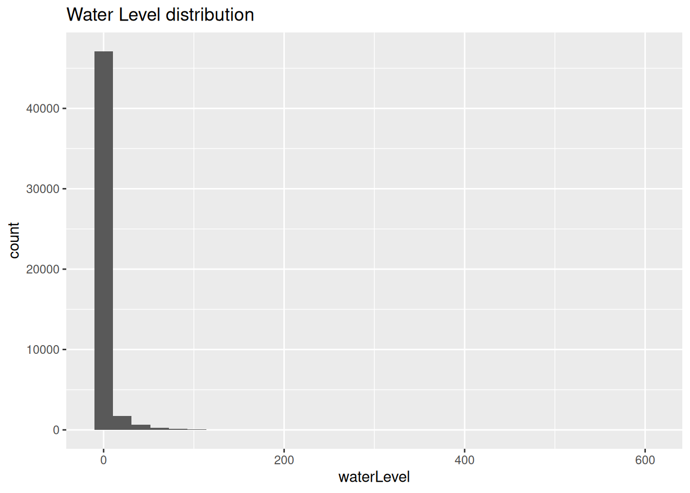
df_test %>%
mutate(waterLevel=as.numeric(waterLevel)) %>%
ggplot(aes(x=waterLevel)) +
geom_histogram() +
labs(
title="Water Level distribution"
)
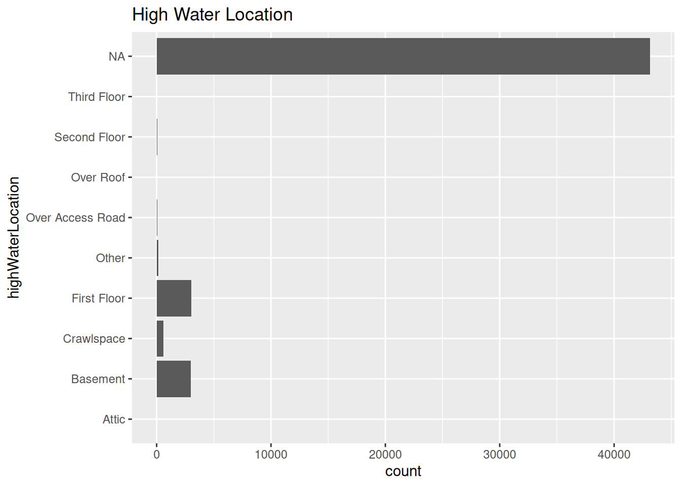
df_test %>%
ggplot(aes(x=highWaterLocation)) +
geom_bar() +
coord_flip() +
labs(
title="High Water Location"
)
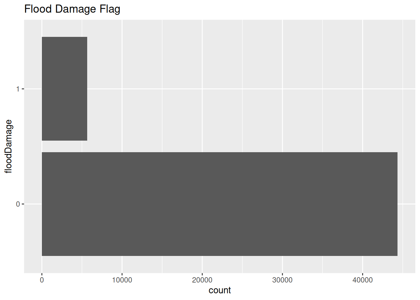
df_test %>%
ggplot(aes(x=floodDamage)) +
geom_bar() +
coord_flip() +
labs(
title="Flood Damage Flag"
)
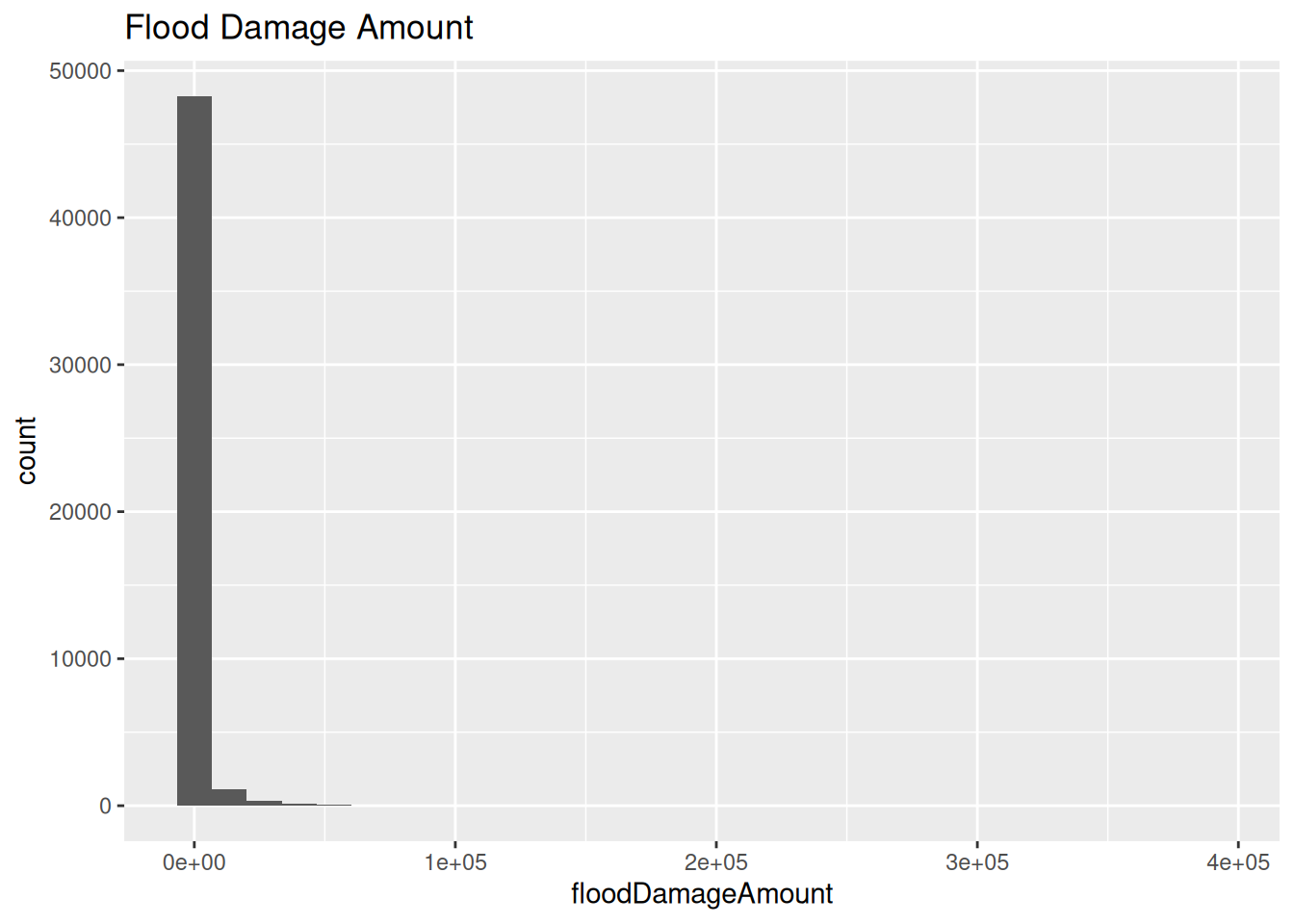
df_test %>%
mutate(floodDamageAmount=as.numeric(floodDamageAmount)) %>%
ggplot(aes(x=floodDamageAmount)) +
geom_histogram() +
labs(
title="Flood Damage Amount"
)
# make a table
Damages <- tribble(~Variable, ~Flood)
Damages_value <- df_test %>%
mutate(waterLevel=as.numeric(waterLevel)) %>%
filter(waterLevel>0) %>%
count()
Damages[1,]$Variable <- "Water Level"
Damages[1,]$Flood <- Damages_value$n[1]
Damages_value <- df_test %>%
filter(!is.na(highWaterLocation)) %>%
count()
Damages[2,]$Variable <- "High Water Location"
Damages[2,]$Flood <- Damages_value$n[1]
Damages_value <- df_test %>%
filter(floodDamage=="1") %>%
count()
Damages[3,]$Variable <- "Flood Damage Flag"
Damages[3,]$Flood <- Damages_value$n[1]
Damages_value <- df_test %>%
mutate(floodDamageAmount=as.numeric(floodDamageAmount)) %>%
filter(floodDamageAmount>0) %>%
count()
Damages[4,]$Variable <- "Flood Damage Value"
Damages[4,]$Flood <- Damages_value$n[1]
Damages %>%
gt()| Variable | Flood |
|---|---|
| Water Level | 6718 |
| High Water Location | 6868 |
| Flood Damage Flag | 5633 |
| Flood Damage Value | 5468 |
# Look at combinations
foo <- df_test %>%
filter(!is.na(highWaterLocation))
df_test %>%
mutate(floodDamageAmount=as.numeric(floodDamageAmount)) %>%
filter(floodDamageAmount>0) %>%
filter(floodDamage=="0") # A tibble: 0 × 71
# ℹ 71 variables: incidentType <chr>, declarationDate <date>,
# disasterNumber <chr>, county <chr>, damagedStateAbbreviation <chr>,
# damagedCity <chr>, damagedZipCode <chr>, applicantAge <chr>,
# householdComposition <chr>, occupantsUnderTwo <chr>, occupants2to5 <chr>,
# occupants6to18 <chr>, occupants19to64 <chr>, occupants65andOver <chr>,
# grossIncome <chr>, ownRent <chr>, primaryResidence <chr>,
# residenceType <chr>, homeOwnersInsurance <chr>, floodInsurance <chr>, …# Nothing from above. But there can be flagged flood damage with a $0 amount.Lets look at some simple statistics
Some abbreviations:
| Abbrev | Full Name |
|---|---|
| IHP | Individual Housing Program |
| HA | Housing Assistance |
| ONA | Other Needs Assistance |
| TSA | Transitional Sheltering Assistance |
# top 10 states for number of applications
df2 %>%
group_by(damagedStateAbbreviation) %>%
summarize(Applications=n(),
Accepted=sum(ihpEligible|haEligible|onaEligible|tsaEligible)) %>%
ungroup() %>%
mutate(Rejected=Applications-Accepted) %>%
arrange(desc(Applications)) %>%
rename(State=damagedStateAbbreviation) %>%
head(10) %>%
mutate(State = fct_reorder(State, Applications)) %>%
select(-Applications) %>%
pivot_longer(!State, names_to = "Status", values_to = "Applications") %>%
ggplot(aes(y=Applications, x=State, fill=Status)) +
geom_col() +
scale_y_continuous(labels = scales::label_comma())+
scale_fill_manual(values =c('green','red')) +
coord_flip() +
labs(title="Number of Flood Disaster Assistance Applications by State",
subtitle="From 2002 until March 2025, Top Ten")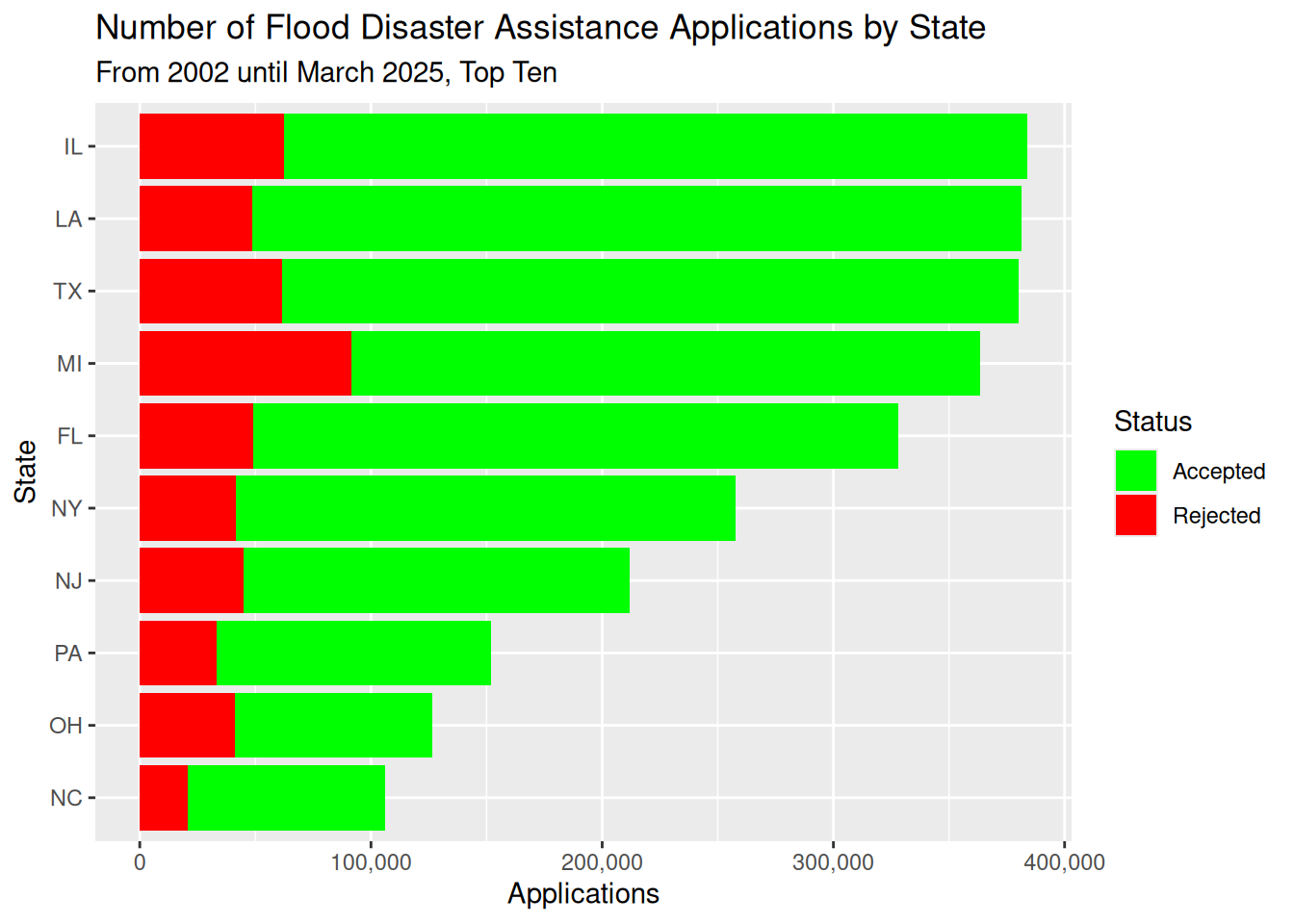
# top 10 zipcodes for number of applications
df2 %>%
group_by(damagedZipCode) %>%
summarize(Applications=n(),
Accepted=sum(ihpEligible|haEligible|onaEligible|tsaEligible),
State=first(damagedStateAbbreviation)) %>%
ungroup() %>%
mutate(Rejected=Applications-Accepted) %>%
arrange(desc(Applications)) %>%
rename(Zip=damagedZipCode) %>%
head(10) %>%
mutate(Zip=paste(Zip, '-', State)) %>%
mutate(Zip = fct_reorder(Zip, Applications)) %>%
select(-Applications, -State) %>%
pivot_longer(!Zip, names_to = "Status", values_to = "Applications") %>%
ggplot(aes(y=Applications, x=Zip, fill=Status)) +
geom_col() +
scale_y_continuous(labels = scales::label_comma())+
scale_fill_manual(values =c('green','red')) +
coord_flip() +
labs(title="Number of Flood Disaster Assistance Applications by Zip",
subtitle="From 2002 until March 2025, Top Ten")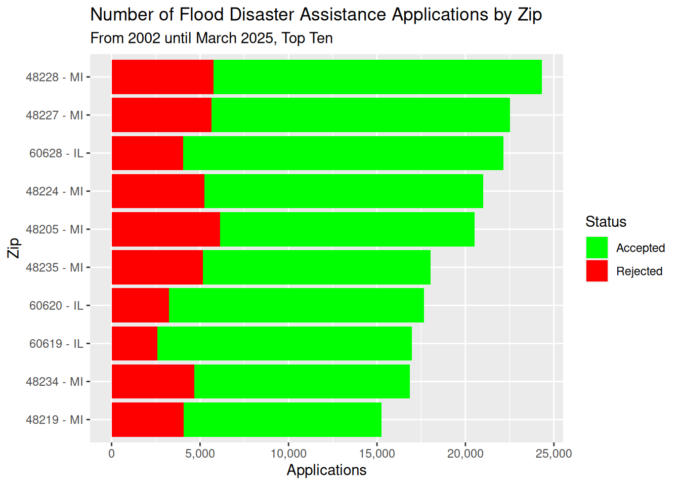
# top 10 zipcodes for number of disasters
df2 %>%
group_by(damagedZipCode) %>%
summarize(Applications=n(),
Floods=as.integer(n_distinct(declarationDate)),
State=first(damagedStateAbbreviation)
) %>%
ungroup() %>%
arrange(desc(Floods), desc(Applications)) %>%
rename(Zip=damagedZipCode) %>%
head(15) %>%
mutate(Zip=paste(Zip, '-', State)) %>%
mutate(Zip = fct_reorder(Zip, Applications)) %>%
select(-State) %>%
mutate(Floods=fct(as.character(Floods))) %>%
ggplot(aes(y=Applications, x=Zip, fill=Floods)) +
geom_col() +
scale_y_continuous(labels = scales::label_comma())+
scale_fill_manual(values =c('#F0E442','#0072B2', "green"), name="# Floods") +
coord_flip() +
labs(title="Number of Flood Disaster Assistance Applications by Zip",
subtitle="From 2002 until March 2025, top fifteen by number of floods")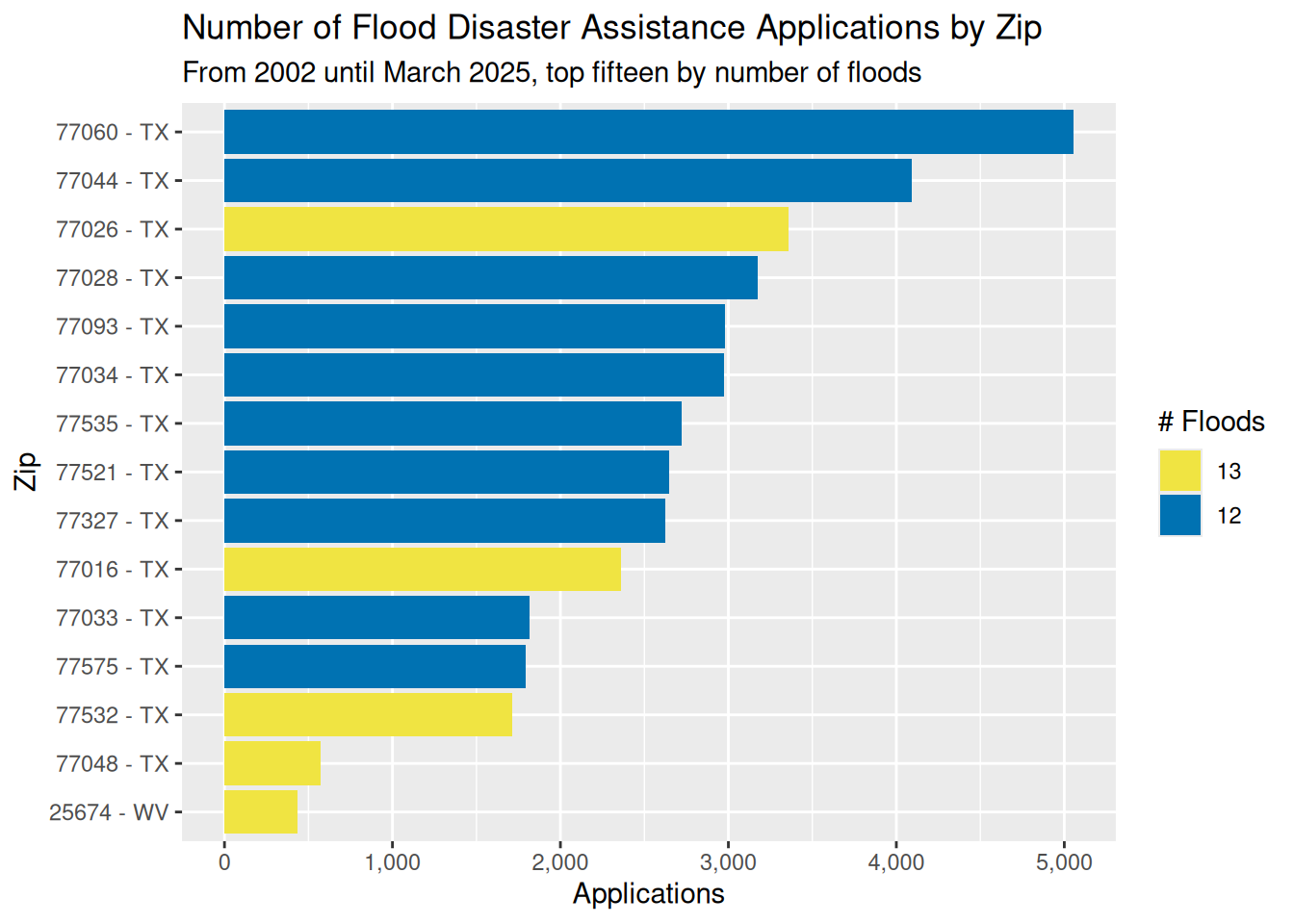
# Distribution of # floods by zipcode
df2 %>%
group_by(damagedZipCode) %>%
summarize(Applications=n(),
Floods=n_distinct(declarationDate),
State=first(damagedStateAbbreviation)
) %>%
ungroup() %>%
rename(Zip=damagedZipCode) %>%
ggplot(aes(x=Floods)) +
geom_histogram(bins=13) +
labs(title="Number of Flood Events by Zip Code",
subtitle="From 2002 until March 2025",
x="Number of Flood Events",
y="Number of Zip Codes")
Let’s make a map of number of flood events, for # > 4
foo <- df2 %>%
group_by(damagedZipCode) %>%
summarize(Applications=n(),
Floods=n_distinct(declarationDate),
State=first(damagedStateAbbreviation)
) %>%
ungroup() %>%
filter(Floods>4) %>%
filter(State!="PR") %>% # Drop Puerto Rico
rename(Zip=damagedZipCode)
# Get zipcode polygons
ZCTA_geom <- readRDS(paste0(datapath, "ZCTA_geometry.rds"))
foo2 <- left_join(foo, ZCTA_geom, by=join_by(Zip==GEOID)) %>%
select(-NAME, -variable, -estimate, -moe) %>%
sf::st_as_sf() %>%
sf::st_transform(crs=googlecrs)
# make map
pal <- colorNumeric("YlOrBr",
c(min(foo2$Floods, na.rm=TRUE),
max(foo2$Floods, na.rm=TRUE)),
na.color = "transparent")
map <- leaflet(data=foo2) %>% addTiles() %>%
addPolygons(data=foo2,
weight=2,
color="black",
fillColor = pal(foo2$Floods),
popup = paste(
"<div class='leaflet-popup-scrolled' style='max-width:150px;max-height:200px'>",
"Zip code:", foo2$Zip, "<br>",
"Applications:", foo2$Applications, "<br>",
"# of floods:", foo2$Floods,
"</div>"
))
map