#   A better mode function
Mode <- function(x) {
  ux <- unique(x)
  ux[which.max(tabulate(match(x, ux)))]
}

#   Add to cleanup

add_Clean <- function(df, filt, remain, old) {
  drop <- old - remain
  df %>%
    add_row(Filter=filt,
            Remaining=remain,
            Dropped=drop)
}Fema Flood Data
Mapping
Supporting Activism
Episcopal Relief and Development
Developing a tool to find poor neighborhoods that flood frequently
Create a clean version of FEMA’s flood claims file
This is a project for Episcopal Relief and Development. The goal is to identify poor neighborhoods subject to frequent flooding, so that ERD can try to help people move out of those areas to safer locations. So we need to look at historical flooding data, and combine that with census and social vulnerability data.
FEMA has a parquet file where each record documents a flood claim made. The file begins in 1978, and goes up until 2025. It contains many data fields, but in particular has the census Block Group, as well as much information about the nature of the flood, the structure, the claim, and some demographic data.
https://www.fema.gov/openfema-data-page/fima-nfip-redacted-claims-v2
Functions
Set up connection to file and read and save
FEMA <- arrow::open_dataset(paste0(pq_path,"FimaNfipClaims (2).parquet"))

FEMA_all <- FEMA %>% collect()

saveRDS(FEMA_all, paste0(path, "FEMA/FEMA_Flood.rds"))

Cleanup <- add_Clean(Cleanup, "Original", nrow(FEMA_all), nrow(FEMA_all))
Clean up data
I want to collapse the data to Block-Group level statistics. But I also want to retain the flood events that have hit each block, and do some filtering. I don’t care about floods that generated only 1 or 2 claims, for example.
Unfortunately, the block group may be derived from the 2010 or the 2020 census for each record, and there is no way to actually know. I will try to get close and assume that for each record last updated before 2020, that they used the 2010 census, and then take a close look at the post 2020 data.
#   Select potentially interesting fields and select occupancy types

###   causeOfDamage:
# 0 : Other causes;
# 1 : Tidal water overflow;
# 2 : Stream, river, or lake overflow;
# 3 : Alluvial fan overflow;
# 4 : Accumulation of rainfall or snowmelt;
# 7 : Erosion-demolition;
# 8 : Erosion-removal;
# 9 : Earth movement, landslide, land subsidence, sinkholes, etc.

###   occupancyType:
# 1 = single family residence;
# 2 = 2 to 4 unit residential building;
# 3 = residential building with more than 4 units;
# 4 = Non-residential building;
# 6 = Non Residential - Business;
# 11 = Single-family residential building with the exception of a mobile home or a single residential unit within a multi unit building;
# 12 = A residential non-condo building with 2, 3, or 4 units seeking insurance on all units;
# 13 = A residential non-condo building with 5 or more units seeking insurance on all units;
# 14 = Residential mobile/manufactured home;
# 15 = Residential condo association seeking coverage on a building with one or more units;
# 16 = Single residential unit within a multi-unit building;
# 17 = Non-residential mobile/manufactured home;
# 18 = A non-residential building;
# 19 = a non-residential unit within a multi-unit building

FEMA2 <- FEMA_all %>%
  select(asOfDate, dateOfLoss, state, countyCode, ratedFloodZone, occupancyType,
         amountPaidOnBuildingClaim, amountPaidOnContentsClaim, yearOfLoss,
         buildingDamageAmount, primaryResidenceIndicator,
         rentalPropertyIndicator, buildingPropertyValue,
         buildingReplacementCost, causeOfDamage, floodEvent, waterDepth,
         floodZoneCurrent, censusTract, censusBlockGroupFips, nfipCommunityName,
         eventDesignationNumber, latitude, longitude) %>%
  arrange(dateOfLoss)  %>%
  filter(occupancyType %in% c(1,2,3,11,12,13,14,15)) # residential only

Cleanup <- add_Clean(Cleanup, "Drop Non-residential", nrow(FEMA2), nrow(FEMA_all))


#   Let's look at the distribution of some of the values to see how valuable they
#   actually might be.

NA_count <- modify(FEMA2, ~sum(is.na(.)))
NA_count <- pivot_longer(NA_count[1,],
                         everything(),
                         names_to="Variable",
                         values_to="Num_NA")
NA_count %>%
  mutate(Pct=Num_NA/nrow(FEMA2)) %>%
  gt() %>%
    fmt_number(
      columns = everything(),
      decimals=0,
      use_seps = TRUE
)| Variable | Num_NA | Pct |
|---|---|---|
| asOfDate | 0 | 0 |
| dateOfLoss | 0 | 0 |
| state | 0 | 0 |
| countyCode | 54,461 | 0 |
| ratedFloodZone | 124,590 | 0 |
| occupancyType | 0 | 0 |
| amountPaidOnBuildingClaim | 524,061 | 0 |
| amountPaidOnContentsClaim | 524,061 | 0 |
| yearOfLoss | 0 | 0 |
| buildingDamageAmount | 543,743 | 0 |
| primaryResidenceIndicator | 0 | 0 |
| rentalPropertyIndicator | 0 | 0 |
| buildingPropertyValue | 543,743 | 0 |
| buildingReplacementCost | 543,743 | 0 |
| causeOfDamage | 33,485 | 0 |
| floodEvent | 672,141 | 0 |
| waterDepth | 216,563 | 0 |
| floodZoneCurrent | 1,764,729 | 1 |
| censusTract | 119,120 | 0 |
| censusBlockGroupFips | 119,120 | 0 |
| nfipCommunityName | 1,719,582 | 1 |
| eventDesignationNumber | 2,302,482 | 1 |
| latitude | 36,585 | 0 |
| longitude | 36,585 | 0 |
##    Clearly some variables are useless

#   We have more lat longs than we have counties and census blocks. Do we want
#   to use that?

No_county <- FEMA2 %>%
  filter(is.na(countyCode)) %>%
  group_by(state) %>%
    summarize(No_lat=sum(is.na(latitude)),
              lat=sum(!is.na(latitude)),
              NoBlkgrp=sum(is.na(censusBlockGroupFips)),
              Blkgrp=sum(!is.na(censusBlockGroupFips)))

#   Look at primaryResidenceIndicator, If not a primary residence (vacation home)
#   then don't care

Residence_indicator <- FEMA2 %>%
  group_by(state) %>%
  summarize(Primary=sum(primaryResidenceIndicator==TRUE),
            Not_primary=sum(primaryResidenceIndicator==FALSE)) %>%
  select(state, Primary, Not_primary)

FEMA2 %>%
  summarize(Primary=sum(primaryResidenceIndicator==TRUE),
            Not_primary=sum(primaryResidenceIndicator==FALSE),
            Rental=sum(rentalPropertyIndicator==TRUE),
            Not_rental=sum(rentalPropertyIndicator==FALSE)) %>%
  gt() %>%
    fmt_number(
      columns = everything(),
      decimals=0,
      use_seps = TRUE
)| Primary | Not_primary | Rental | Not_rental |
|---|---|---|---|
| 1,323,791 | 1,144,573 | 29,944 | 2,438,420 |
FEMA2 %>%
  summarize(Primary_rental=sum(primaryResidenceIndicator&rentalPropertyIndicator),
            Primary_nonRent=sum(primaryResidenceIndicator&(!rentalPropertyIndicator)),
            NonPri_rental=sum((!primaryResidenceIndicator)&rentalPropertyIndicator),
            NonPri_Nonrent=sum((!primaryResidenceIndicator)&(!rentalPropertyIndicator))) %>%
  gt() %>%
    fmt_number(
      columns = everything(),
      decimals=0,
      use_seps = TRUE
)| Primary_rental | Primary_nonRent | NonPri_rental | NonPri_Nonrent |
|---|---|---|---|
| 2,679 | 1,321,112 | 27,265 | 1,117,308 |
#   Drop if missing state, county, or block group (about 120,000 records)

old <- nrow(FEMA2)

FEMA2 <- FEMA2 %>%
  filter(!state=="UN", # unknown
         !state=="VI", # Virgin Islands
         !state=="GU", # Guam
         !is.na(censusBlockGroupFips),
         !is.na(countyCode))

Cleanup <- add_Clean(Cleanup, "Missing BlkGrp, Guam, V.I.", nrow(FEMA2), old)
old <- nrow(FEMA2)
# Note that lat, longs are not useful - they have 1 decimal, so are
# accurate to about 7 miles.
Drop_columns <- c("floodZoneCurrent", "censusTract", "eventDesignationNumber",
"latitude", "longitude")
FEMA2 <- FEMA2 %>%
# Drop a few more variables and create a few
select(-one_of(Drop_columns)) %>%
mutate(Month=lubridate::month(dateOfLoss, label=TRUE)) %>%
mutate(Occupancy=case_when(
occupancyType==1 | occupancyType==11 | occupancyType==15 ~ "Own",
occupancyType==14 ~ "Mobile",
.default="Rent"
))census block group problem - crosswalk where possible
I don’t know which census was used to derive the block groups. And there is no good way to recover that information. So I will make a few assumptions, try to put what records I can onto 2020 census block groups, and toss the rest.
Note that the crosswalk file was downloaded from the Census website shortly before the great data purge began.
#   Let's look at the census block group problem

States <- unique(FEMA2$state)
Cpath <- "/home/ajackson/Dropbox/Rprojects/Curated_Data_Files/Census_data/Flood/"
Xpath <- "/home/ajackson/Dropbox/Rprojects/ERD/Data/"

Xwalk <- read_delim(paste0(Xpath, "tab20_blkgrp20_blkgrp10_natl.txt"),
                    delim="|", col_types="cccnncccccnnccnn") %>%
          select(GEOID_BLKGRP_20, GEOID_BLKGRP_10, AREALAND_PART,
                 AREALAND_BLKGRP_20, AREALAND_BLKGRP_10)

#   Same blk grp id *and* large overlap - these have barely changed
Same <- Xwalk %>%
  filter(GEOID_BLKGRP_20==GEOID_BLKGRP_10) %>%
  mutate(Overlap=AREALAND_PART/AREALAND_BLKGRP_10) %>%
  filter(Overlap>=0.9)

#   Largeish overlap, not equal ids. Names changed, but boundaries similar
Xwalk2 <- Xwalk %>%
  filter(AREALAND_PART>0) %>%
  group_by(GEOID_BLKGRP_10) %>%
      reframe(Overlap=AREALAND_PART/AREALAND_BLKGRP_10,
              GEOID_BLKGRP_20=first(GEOID_BLKGRP_20, order_by=AREALAND_PART),
              Num_10=n()
              ) %>%
  filter(Overlap>0.8) %>%
  filter(GEOID_BLKGRP_20!=GEOID_BLKGRP_10)

for (astate in States) {
  Census2020 <- readRDS(paste0(Cpath, "ACS_", astate, ".rds"))
  Census2020_nogeom <- Census2020 %>% sf::st_drop_geometry() %>%
    select(GEOID, Pop_acs)

  #   if asOfDate is prior to 2020, then it seems likely that the 2010 census was used

  FEMA2_early <- FEMA2 %>% #    pull out data prior to 2020
    filter(asOfDate<lubridate::mdy("1/1/2020")) %>%
    filter(state==astate)
  FEMA2_late <- FEMA2 %>%
    filter(asOfDate>=lubridate::mdy("1/1/2020")) %>%
    filter(state==astate)

  #   Match late records to 2020 census, and pull out the non-matches.

  Late_BlkGrps <- FEMA2_late %>%
    left_join(., Census2020_nogeom, by=join_by("censusBlockGroupFips"=="GEOID"))

  Remainder <- Late_BlkGrps %>%
    filter(is.na(Pop_acs)) %>% select(-Pop_acs)

  Late_BlkGrps <- Late_BlkGrps %>%
    filter(!is.na(Pop_acs)) %>% select(-Pop_acs)

  #   Match early records to "Same" and then match to 2020 census

  Good_early <- FEMA2_early %>%
    left_join(., Same, by=join_by("censusBlockGroupFips"=="GEOID_BLKGRP_20")) %>%
    select(-GEOID_BLKGRP_10, -starts_with("AREA"))

  Remainder2 <- Good_early %>%
    filter(is.na(Overlap)) %>% select(-Overlap)

  Good_early <- Good_early %>%
    filter(!is.na(Overlap)) %>% select(-Overlap)

  #   Combine Remainder files and cross walk them

  Remainder <- bind_rows(Remainder, Remainder2)

  Remainder <- Remainder %>%
    filter(!is.na(censusBlockGroupFips))

  New_remainder <- Remainder %>%
    inner_join(., Xwalk2, by=c("censusBlockGroupFips"="GEOID_BLKGRP_10")) %>%
    mutate(censusBlockGroupFips=GEOID_BLKGRP_20) %>%
    select(-Overlap, -Num_10, -GEOID_BLKGRP_20)

  Final <- bind_rows(Late_BlkGrps, Good_early, New_remainder)

  saveRDS(Final, paste0(Xpath, "Xwalk/FEMA_", astate, ".rds"))

}
Collapse data by block group, filter and add geometry
FEMA1 <- readRDS(paste0(Xpath, "Xwalk/FEMA_", States[1], ".rds"))
for (state in States[2:length(States)]) {
  FEMA1 <- bind_rows(FEMA1, readRDS(paste0(Xpath, "Xwalk/FEMA_", state, ".rds")))
}

Cleanup <- add_Clean(Cleanup, "After attaching census data", nrow(FEMA1), old)
old <- nrow(FEMA1)

#   Filter out low impact events (# claims for a primary in a blk grp <1)

#             Create a list of week_yr per blk grp to keep
Keep_list <- FEMA1 %>%
  replace_na(list(nfipCommunityName="Unk")) %>% # replace NA with Unk
  replace_na(list(floodEvent="Unk")) %>% # replace NA with Unk
  # Create a 1 week window to try to capture a single event
  mutate(week_yr=paste(lubridate::year(dateOfLoss-3),
                       lubridate::week(dateOfLoss-3))) %>%
  group_by(censusBlockGroupFips, week_yr) %>%
    summarize(Num_primary=sum(primaryResidenceIndicator),
              Flood_event=Mode(floodEvent),
              yearOfLoss=first(yearOfLoss),
              Month=first(Month)) %>%
  ungroup()

old <- nrow(Keep_list)
Cleanup <- add_Clean(Cleanup, "Collapse by BlkGrp and Event", nrow(Keep_list), old)


Keep_list %>%
  filter(Num_primary<15) %>% # so it's easier to see stuff
  ggplot(aes(x=Num_primary)) +
  geom_histogram(binwidth = 1) +
  labs(title="Total Claims (Primary) Distribution",
       x="# Primary Claims per event",
       y="Number")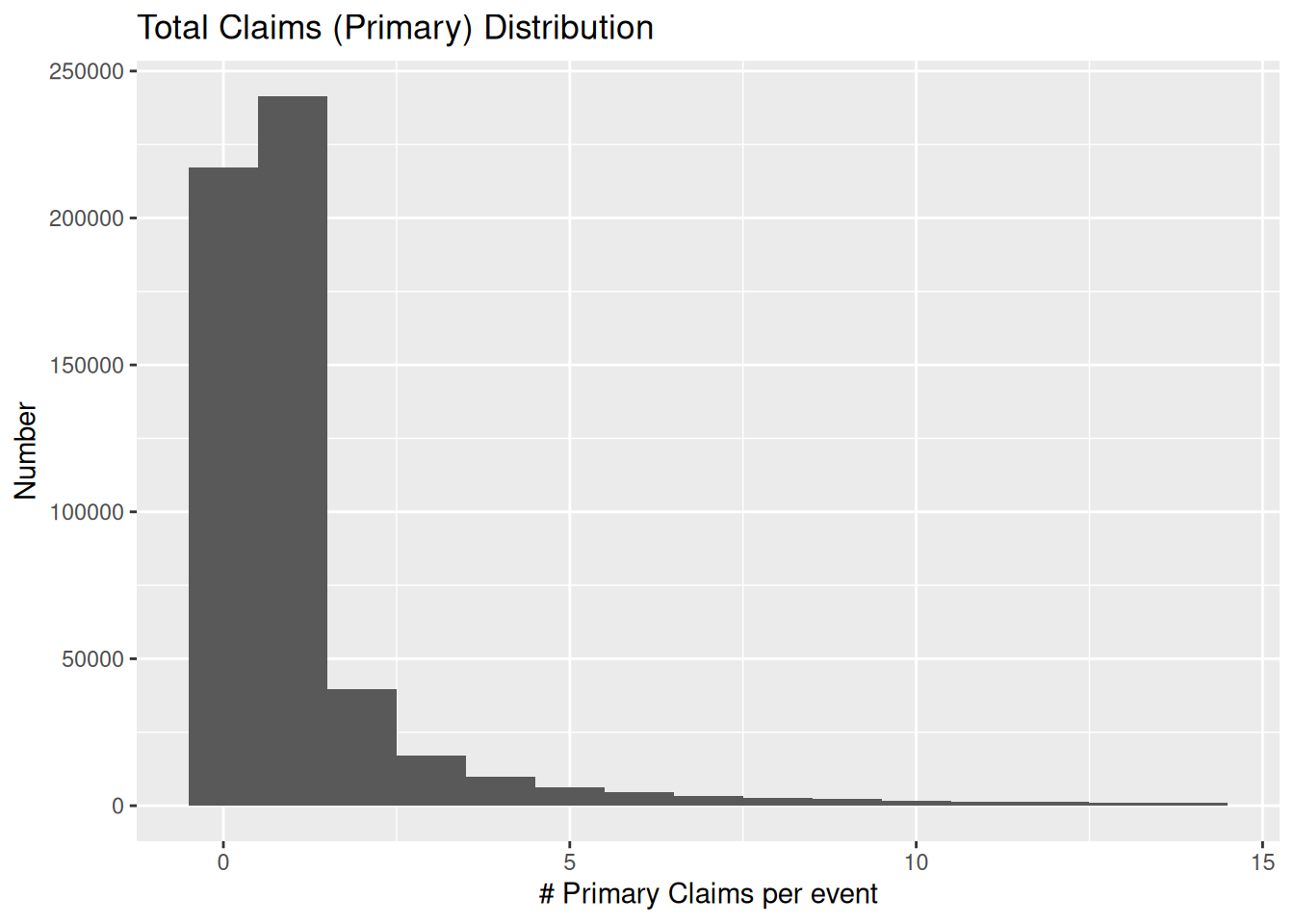
Keep_list <- Keep_list %>%
  filter(Num_primary>0) # need at least 1 claim on primary residence per event

Cleanup <- add_Clean(Cleanup, "BlkGrp needs >0 Primary Homes", nrow(Keep_list), old)
old <- nrow(Keep_list)

#   Collapse data by GEOID

FEMA4 <- FEMA1 %>%
  replace_na(list(nfipCommunityName="Unk")) %>% # replace NA with Unk
  # Create a 1 week window to try to capture a single event
  mutate(week_yr=paste(lubridate::year(dateOfLoss-3),
                       lubridate::week(dateOfLoss-3))) %>%
  #   Drop values with <5 primary residence claims for a given event
  inner_join(., Keep_list, join_by(censusBlockGroupFips, week_yr)) %>%
  #   Calculate blk grp statistics
  group_by(censusBlockGroupFips, Occupancy, primaryResidenceIndicator) %>%
    summarise(Num_Claims=n(),
              Num_dates=n_distinct(week_yr),
              State=first(state),
              County=first(countyCode)) %>%
  ungroup() %>%
  pivot_wider(names_from = Occupancy, values_from = c(Num_Claims, Num_dates),
              values_fill=0) %>%
  replace_na(list(Num_Claims_Mobile=0,
                  Num_dates_Mobile=0)) %>%
  mutate(Num_Claims=Num_Claims_Own+Num_Claims_Rent+Num_Claims_Mobile,
         Num_dates=Num_dates_Own+Num_dates_Rent+Num_dates_Mobile)

#   widen by combining primary residence indicator records

Foobar <- FEMA4 %>%
  mutate(Residence=if_else(primaryResidenceIndicator, "Primary", "Vacation")) %>%
  select(-primaryResidenceIndicator) %>%
  pivot_wider(names_from=Residence, values_from = starts_with("Num_")) %>%
  select(-Num_Claims_Own_Vacation, -Num_Claims_Rent_Vacation,
         -Num_Claims_Mobile_Vacation, -Num_dates_Own_Vacation,
         -Num_dates_Rent_Vacation, -Num_dates_Mobile_Vacation, -Num_dates_Vacation,
         -Num_dates_Own_Primary, -Num_dates_Rent_Primary, -Num_dates_Mobile_Primary) %>%
  filter(!is.na(Num_Claims_Primary)) #    Drop where only vacation homes claimed

old <- nrow(FEMA4)
Cleanup <- add_Clean(Cleanup, "Collapse to BlkGrps and drop only vacation homes", nrow(Foobar), old)

#   Look at long storm names to shorten them

Storm_names <- FEMA1$floodEvent %>% unique()
foo <- Storm_names[order(nchar(Storm_names), Storm_names)] # look at names

#   Pull out storm names to later add back to file

Storms <- Keep_list %>%
  filter(!is.na(censusBlockGroupFips)) %>%
  mutate(Flood_event=stringr::str_replace(Flood_event, "Hurricane ", "H. ")) %>%
  mutate(Flood_event=stringr::str_replace(Flood_event, "Tropical Storm", "T.S.")) %>%
  mutate(Flood_event=stringr::str_replace(Flood_event, "Thunderstorms", "T-Storms")) %>%
  mutate(Flood_event=paste(Flood_event, yearOfLoss, Month)) %>%
  #   Create strings of the storm names/year/month and the number of homes flooded
  group_by(censusBlockGroupFips) %>%
    summarize(floodEvents=paste(Flood_event, collapse=", "),
              floodNum=paste(Num_primary,collapse=", ")) %>%
  ungroup()

Final_FEMA <-  Foobar %>%
  inner_join(., Storms, by="censusBlockGroupFips") %>%
  filter(!State=="UN") %>%
  filter(Num_Claims_Primary>9) # 10 or more claims total

old <- nrow(Foobar)
Cleanup <- add_Clean(Cleanup, "10 or more claims only", nrow(Final_FEMA), old)

saveRDS(Final_FEMA, paste0(pq_path, "Final_FEMA_by_BlkGrp.rds"))

# causeOfDamage:
# 0 : Other causes;
# 1 : Tidal water overflow;
# : Stream, river, or lake overflow;
# 3 : Alluvial fan overflow;
# 4 : Accumulation of rainfall or snowmelt;
# 7 : Erosion-demolition;
# 8 : Erosion-removal;
# 9 : Earth movement, landslide, land subsidence, sinkholes, etc.


###   occupancy types
# 1=single family residence;
# 2 = 2 to 4 unit residential building;
# 3 = residential building with more than 4 units;
# 4 = Non-residential building;
# 6 = Non Residential - Business;
# 11 = Single-family residential building with the exception of a mobile home or a single residential unit within a multi unit building;
# 12 = A residential non-condo building with 2, 3, or 4 units seeking insurance on all units;
# 13 = A residential non-condo building with 5 or more units seeking insurance on all units;
# 14 = Residential mobile/manufactured home;
# 15 = Residential condo association seeking coverage on a building with one or more units;
# 16 = Single residential unit within a multi-unit building;
# 17 = Non-residential mobile/manufactured home;
# 18 = A non-residential building;
# 19 = a non-residential unit within a multi-unit building;
Attach census and vulnerability data by state
#   Look at distribution of flood events per block group

Final_FEMA %>%
  ggplot(aes(x=Num_dates_Primary)) +
  geom_histogram(binwidth = 1) +
  labs(title="Total Flood Events Distribution",
       x="Flood events per block group",
       y="Number")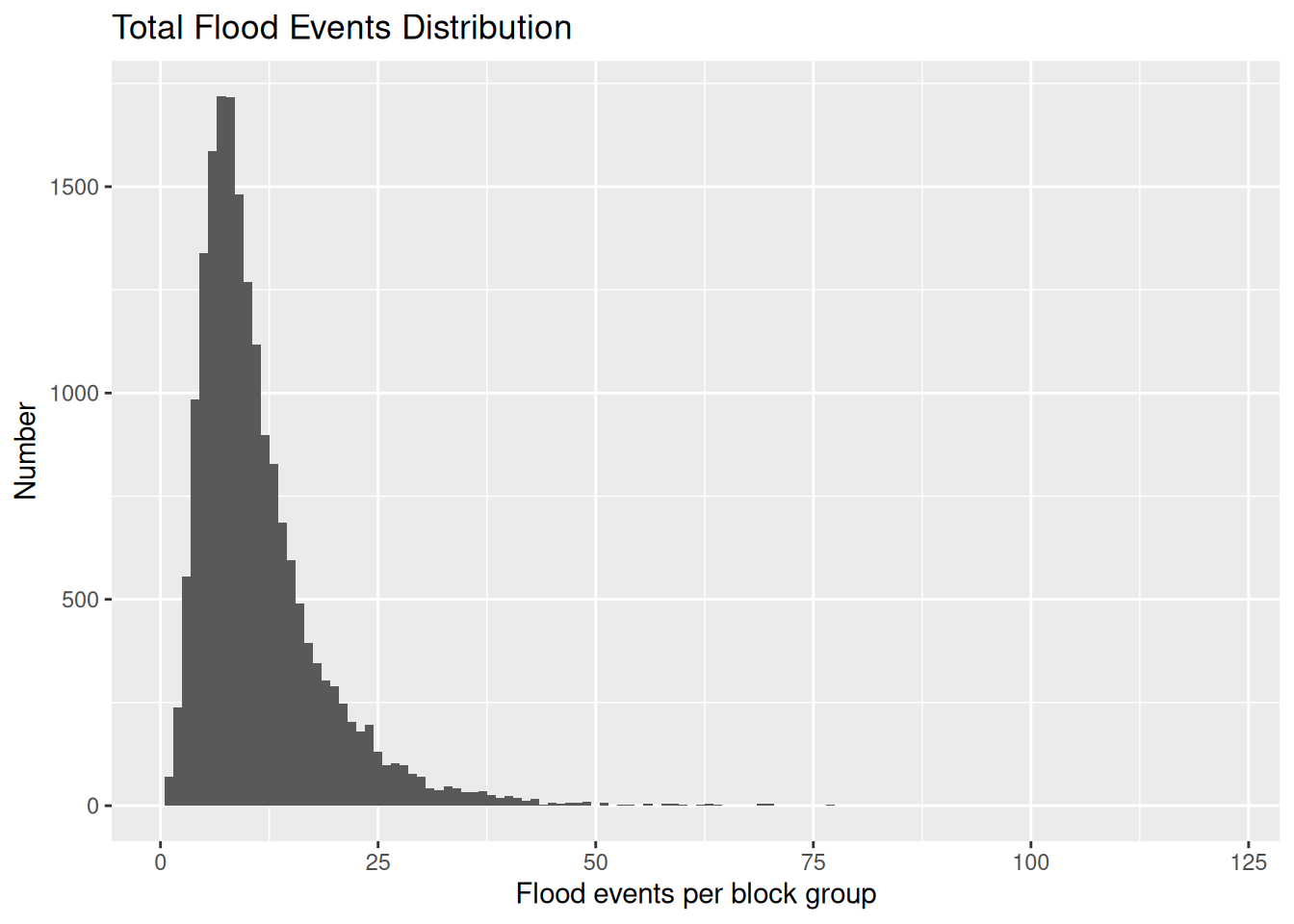
#   First drop any blocks with fewer than 3 distinct flood events

Final_FEMA_short <- Final_FEMA %>%
  filter(Num_dates_Primary>2)

old <- nrow(Final_FEMA)
Cleanup <- add_Clean(Cleanup, "Must have >2 flood events", nrow(Final_FEMA_short), old)

#   Attach census and vulnerability data by state

astate <- "AL"
new <- 0  # count remaining rows
for (astate in unique(Final_FEMA_short$State)) {
  if(astate=="PR") {next} #   No vuln index there
  # print(astate)
  Census <- readRDS(paste0(path, "Census_data/Flood/ACS_", astate, ".rds"))

  Vuln <- readRDS(paste0(path, "SocialVulnIndex/SVI_", astate, ".rds")) %>%
    select(-year, -state) %>%
    mutate(RPL_theme1=signif(RPL_theme1,2),
           RPL_theme2=signif(RPL_theme2,2),
           RPL_theme3=signif(RPL_theme3,2),
           RPL_theme4=signif(RPL_theme4,2),
           RPL_themes=signif(RPL_themes,2)) %>%
    rename(c(Socio_Econ=RPL_theme1,
             Household_Ages=RPL_theme2,
             Ethnicity=RPL_theme3,
             Housing=RPL_theme4,
             Vuln_Index=RPL_themes))

  #   Attach vulnerability indicies

  foo <- Final_FEMA_short %>%
    mutate(GEOID=stringr::str_sub(censusBlockGroupFips, 1, 11)) %>%
    inner_join(., Vuln, by="GEOID") %>%
    select(-GEOID)

  # attach census data and the geometry

  foo <- foo %>%
    inner_join(., Census, join_by(censusBlockGroupFips == GEOID)) %>%
    sf::st_as_sf()

  #   Drop block groups where percent of households in poverty is <25%

  foo <- foo %>%
    filter(Pct_poverty>=25)

  new <- new + nrow(foo)

  #   Calculate Claims per household

  foo <- foo %>%
    mutate(ClaimsPerHousehold=signif(Num_Claims_Primary/Households, 2))

  saveRDS(foo, paste0(pq_path, "Final_FEMA_Flood_Data/FEMA_", astate, ".rds"))
}

old <- nrow(Final_FEMA_short)
Cleanup <- add_Clean(Cleanup, "Poverty households >= 25%", new, old)

Cleanup %>%
  mutate(Group=case_when(row_number()<5 ~ "a",
                         row_number()>6 ~ "c",
                         .default = "b")) %>%
  gt(
    # groupname_col = "Group"
  ) %>%
  tab_header(
    title="Progressive Filtering and Combining"
  ) %>%
  tab_row_group(
    label="Original Claims",
    id = "a",
    rows = Group=="a"
  ) %>%
  tab_row_group(
    label="Collapse to BlkGrp and event",
    id = "b",
    rows = Group=="b"
  ) %>%
  tab_row_group(
    label="Collapse to Only Blk Grps",
    id = "c",
    rows = Group=="c"
  )  %>%
  row_group_order(
    groups=c("a", "b", "c")
  ) %>%
  cols_hide(columns="Group") %>%
  tab_style(
    style = cell_fill(color = "lightgreen"),
    locations = cells_row_groups(groups = c("a", "b", "c"))
  ) %>%
  fmt_number(
    columns=everything(),
    decimals=0
)| Progressive Filtering and Combining | ||
|---|---|---|
| Filter | Remaining | Dropped |
| Original Claims | ||
| Original | 2,704,283 | 0 |
| Drop Non-residential | 2,468,364 | 235,919 |
| Missing BlkGrp, Guam, V.I. | 2,333,084 | 135,280 |
| After attaching census data | 2,223,299 | 109,785 |
| Collapse to BlkGrp and event | ||
| Collapse by BlkGrp and Event | 563,569 | 0 |
| BlkGrp needs >0 Primary Homes | 346,363 | 217,206 |
| Collapse to Only Blk Grps | ||
| Collapse to BlkGrps and drop only vacation homes | 87,840 | 29,002 |
| 10 or more claims only | 18,797 | 69,043 |
| Must have >2 flood events | 18,488 | 309 |
| Poverty households >= 25% | 1,506 | 16,982 |