####################################
#   distance function (Euclidean distance)
####################################

Eucl <- function(x1, x2, y1, y2){sqrt((x1-x2)**2 + (y1-y2)**2)}

####################################
#     Delta dist
####################################
# For each point, take the points before and after and linearly interpolate
# a new point. Then find the distance from that new interpolated point to the
# original. This assumes the input dataframe is an sf file with point geometries.
# I also assume that the data have the acquisition date attached, and so I work
# each date separately to avoid issues with the end of one day trying to connect
# to the beginning of the next

delta_Dist <- function(df){
  df %>%
    mutate(X=sf::st_coordinates(.)[,1],
           Y=sf::st_coordinates(.)[,2]) %>%
    group_by(Date) %>%
      #   Xtest, Ytest are potential new location
      mutate(Xtest=(lag(X, default=first(X)) + lead(X, default=last(X)))/2) %>%
      mutate(Ytest=(lag(Y, default=first(Y)) + lead(Y, default=last(Y)))/2) %>%
      mutate(Dx=Xtest - X,
             Dy=Ytest - Y) %>%
      #   distance from interpolated point to original point
      mutate(Delta_dist=Eucl(Xtest, X, Ytest, Y)) %>%
      #   distance from interpolated point to adjacent points
      mutate(New_dist=Eucl(lag(X, default=first(X)), lead(X, default=last(X)),
                           lag(Y, default=first(Y)), lead(Y, default=last(Y)))/2) %>%
    ungroup()
}

####################################
###   Kalman filter
####################################

# Kalman filter code came from
# https://boazsobrado.com/blog/2017/08/29/implementing-a-kalman-filter-in-r-for-android-gps-measurements/
# which had a few errors (missing asterix's), which I repaired. The variance
# variables were chosen through trial and error.

Kalman <- function(X, Y, varM, varP) {
  # initializing variables
  count <- length(X) # number of data points in the day
  z <- cbind(X,Y) #measurements
  # Allocate space:
  xhat <- matrix(rep(0,2*count),ncol =2) #a posteri estimate at each step
  P <- array(0,dim=c(2,2,count))  #a posteri error estimate
  xhatminus <- matrix(rep(0,2*count),ncol =2) #a priori estimate
  Pminus <- array(0,dim=c(2,2,count)) #a priori error estimate
  K <- array(0,dim=c(2,2,count)) #gain
  # Initializing matrices
  A <-diag(2)
  H<-diag(2)
  R<-function(k) diag(2)* varM[k] #estimate of measurement variance
  Q<-function(k) diag(2)* varP[k] # the process variance
  # initialise guesses:
  xhat[1,] <- z[1,]
  P[,,1] <- diag(2)
  for (k in 2:count){
    # time update
    # project state ahead
    xhatminus[k,] <- A %*% xhat[k-1,]
    # project error covariance ahead
    Pminus[,,k] <- A %*% P[,,k-1] %*%  t(A) + (Q(k))
    # measurement update
    # kalman gain
    K[,,k] <- Pminus[,,k] %*% t(H)/ (H %*% Pminus[,,k] %*% t(H) + R(k))
    # what if NaaN?
    K[,,k][which(is.nan(K[,,k]))]<-0
    # update estimate with measurement
    xhat[k,] <-  xhatminus[k,] + K[,,k] %*% (z[k,] - H %*% xhatminus[k,])
    #update error covariance
    P[,,k] = (diag(2) - K[,,k]%*% H) %*% Pminus[,,k]
  }
  return(as.data.frame(xhat) %>% rename(X2=V1, Y2=V2))
}Cleaning GPS data for Trash Tracker
Mapping
Tracking Litter using a phone app, and mapping the results. This bit is for cleaning up the GPS data.
Trash tracking project
My wife and I like to pick up litter when we walk (which I have learned is called plogging). As part of that I use a nice Android app GPSLogger. It allows me to set up 9 named waypoint buttons, so I can capture the location and type of trash.
However, phone GPS coordinates are notorious for having “issues”. Normal error is around 5 meters, or 16 feet. However, that is the average. There are the occasional points which may be off by a hundred feet or more. The goal of this edition of the blog is to try to eliminate the occasional “spikes”, and to also do some intelligent smoothing to get all the points closer to something reasonable.
For this blog I will look at only one day’s data, just to keep things simple.
Functions
I like to gather the functions together up front, just to keep the code a bit cleaner.
Read in the data
In practice, I read in many files from many days, but for the purposes of this report, I will read in only one day’s worth of data.
#   Read in the files

# in_files <- list.files( path=paste0(path), pattern=".gpx", full.names=TRUE )
df <- NULL

afile <- paste0(path, "20240618.gpx") # June 18 data

# for (afile in in_files) {
  # print(afile)

foo <- XML::htmlTreeParse(afile , useInternalNodes = TRUE)
t_coords <- XML::xpathSApply(doc = foo, path = "//trkpt", fun = XML::xmlAttrs)
t_datetime <- XML::xpathSApply(doc = foo, path = "//trkpt/time", fun = XML::xmlValue)
t_elevation <- XML::xpathSApply(doc = foo, path = "//trkpt/ele", fun = XML::xmlValue)
ways <- XML::xpathSApply(doc = foo, path = "//wpt", fun = XML::xmlAttrs)
wpt_type <- XML::xpathSApply(doc = foo, path = "//wpt/name", fun = XML::xmlValue)
elevation <- XML::xpathSApply(doc = foo, path = "//wpt/ele", fun = XML::xmlValue)
wy_datetime <- XML::xpathSApply(doc = foo, path = "//wpt/time", fun = XML::xmlValue)

#   waypoints first
foo <- data.frame(
  lat = as.numeric(ways["lat", ]),
  lon = as.numeric(ways["lon", ]),
  waypt = wpt_type,
  elevation = as.numeric(elevation),
  dt = lubridate::ymd_hms(wy_datetime)
)

df <- rbind(df, foo)

#   Now track points
foo <- data.frame(
  lat = as.numeric(t_coords["lat", ]),
  lon = as.numeric(t_coords["lon", ]),
  waypt = NA,
  elevation = as.numeric(t_elevation),
  dt = lubridate::ymd_hms(t_datetime)
)

df <- rbind(df, foo)

df <- df %>%
  arrange(dt) %>%
  mutate(Date=as.character(date(dt)))
Preprocess and make a map
First we’ll add a simple geohash (just paste the lat and long together) so that later we can collapse the data where the locations are identical.
We’ll create an sf object (note that the lat longs are on the standard WGS84 datum) and then project them onto a UTM projection appropriate for Seattle (where the data were taken), We don’t want to be doing distance calculations and such in lat long coordinates - we need to be in an X-Y system.
Then we’ll make some plots to see what we have got.
On the map the raw locations are in red, and smoothed locations using a kernel smoother are in green. This shows that we really don’t want to use a kernel smoother. However, we can see that we really need to de-spike the data.
#   add geohash

df$Geohash <- paste(df$lon, df$lat)

#   Collapse identical locations and convert to an sf object

df_sf <- df %>%
  group_by(Date, Geohash) %>%
    summarize(Date=first(Date),
              lat=first(lat),
              lon=first(lon),
              dt=first(dt),
              elevation=first(elevation),
              num=n(),
              waypt=list(waypt)) %>%
  sf::st_as_sf(coords=c("lon","lat"), crs=googlecrs) %>%
  ungroup()

#   Project to UTM, and make X,Y available as variables

df_utm <- sf::st_transform(df_sf, crs=Seattle) %>%
            mutate(X=sf::st_coordinates(.)[,1],
                   Y=sf::st_coordinates(.)[,2]) %>%
            arrange(dt)

#   Show a little data

df_utm %>% sf::st_drop_geometry() %>%
  select(Date, dt, elevation, waypt, X, Y) %>%
  head() %>%
  gt::gt() %>%
gt::tab_header(title="First ten rows")| First ten rows | |||||
|---|---|---|---|---|---|
| Date | dt | elevation | waypt | X | Y |
| 2024-06-18 | 2024-06-18 20:14:43.838 | 1.8000000 | NA | 1279760 | 246347.5 |
| 2024-06-18 | 2024-06-18 20:14:47.645 | 0.3000000 | paper ff, NA | 1279708 | 246417.1 |
| 2024-06-18 | 2024-06-18 20:15:03.746 | 47.9255332 | paper, NA | 1279665 | 246463.5 |
| 2024-06-18 | 2024-06-18 20:15:07.443 | -0.1999999 | plastic, NA | 1279628 | 246477.9 |
| 2024-06-18 | 2024-06-18 20:16:23.846 | -0.1999999 | plastic, NA | 1279649 | 246474.0 |
| 2024-06-18 | 2024-06-18 20:16:39.932 | -11.8471468 | plastic, NA | 1279651 | 246461.8 |
#   Some stats

df_utm %>%
  sf::st_drop_geometry() %>%
  mutate(Dist=Eucl(lag(X, default=first(X)), X,
                   lag(Y, default=first(Y)), Y)) %>%
  filter(Dist<500) %>%
  ggplot(aes(x=Dist)) +
    geom_histogram() +
    labs(title="Distribution of distances between adjacent points",
         x="Distance (ft)",
         y="Number")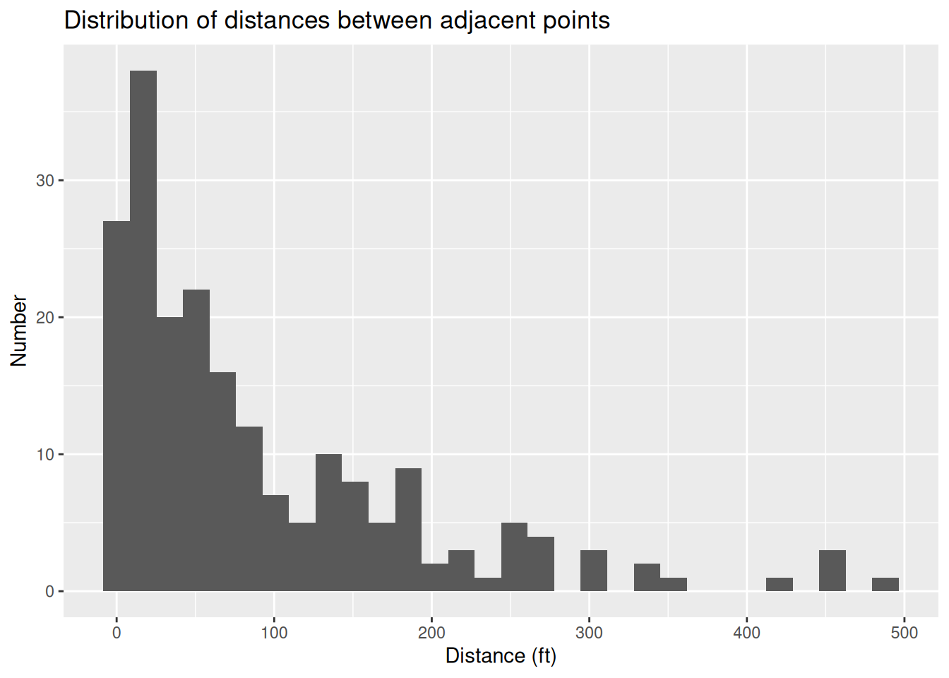
#   Turn into a set of lines

l <- df_utm %>%
  arrange(dt) %>%
  summarize(do_union=FALSE) %>%
  sf::st_cast("LINESTRING")

#   Smooth

ls <- smoothr::smooth(sf::st_geometry(l), method = "ksmooth",
                      smoothness=10)

#   Make a prettier map of path

tmap::tmap_options(basemaps="OpenStreetMap")

tmap::tmap_mode("view") # set mode to interactive plots

tmap::tm_shape(l) +
  tmap::tm_lines(col="red") +
tmap::tm_shape(df_utm %>% select(Date)) +
  tmap::tm_dots(fill="red") +
tmap::tm_shape(ls) +
  tmap::tm_lines(col="green")
Despike the data
Basically for each point we will interpolate a potential replacement from the adjacent points, calculate the distance from the original to the interpolated point, and compare that distance to the distance between the adjacent points. We will choose a threshhold where if exceeded will cause the original point to be replaced.
On the map, green dots are the new coordinates, red are the old points that were changed.
df_utm2 <- delta_Dist(df_utm)

#   Big deltas

#   This value implies we will change values where the distance between the new
#   interpolated value and the original is 160% of the distance between the new
#   point and the adjacent points. For a perfectly straight path, Delta_dist = 0.

Spike_pct <- 1.6 # chosen by trial and error

#   We'll plot this later
df_delta <- df_utm2 %>%
  filter(Delta_dist>Spike_pct*New_dist) %>%
  select(Delta_dist, Date, geometry) %>%
  sf::st_as_sf()

df_utm3 <- df_utm2

for (i in 1:nrow(df_utm3)) {
  if (df_utm3[i,]$Delta_dist>Spike_pct*df_utm3[i,]$New_dist) {
    new_point <- sf::st_point(c(df_utm3[i,]$Xtest, df_utm3[i,]$Ytest)) %>%
                 sf::st_sfc(crs = Seattle)
    df_utm3[i,]$geometry <- sf::st_sfc(sf::st_geometry(new_point))
  }
}

df_delta_after <- df_utm3 %>%
  filter(Delta_dist>Spike_pct*New_dist) %>%
  select(Delta_dist, Date, geometry) %>%
  sf::st_as_sf()

#   Turn into a set of lines

lold <- df_utm2 %>%
  group_by(Date) %>%
  summarize(do_union=FALSE) %>%
  sf::st_cast("LINESTRING")

l <- df_utm3 %>%
  group_by(Date) %>%
  summarize(do_union=FALSE) %>%
  sf::st_cast("LINESTRING")

tmap::tmap_options(basemaps="OpenStreetMap")

tmap::tmap_mode("view") # set mode to interactive plots

tmap::tm_shape(l) +
  tmap::tm_lines(lwd = 2) +
tmap::tm_shape(lold) +
  tmap::tm_lines(col="red") +
tmap::tm_shape(df_delta) +
  tmap::tm_dots(fill="red", size=0.5, popup.vars="Delta_dist")+
tmap::tm_shape(df_delta_after) +
  tmap::tm_dots(fill="green", size=0.5)
Kalman filter
The data is much improved after a simple despike, but it still looks like it could benefit from a bit of intelligent smoothing. We saw earlier that a kernel-based smoothing is not what we want. But for this sort of situation, Kalman filtering is generally what is recommended. I won’t try to explain it - my own understanding is pretty primitive - but that won’t prevent me from using it.
I was able to find a nice example online (see above) with code, for exactly this situation. Unfortunately there are some typos in the code, but I was able to identify them and fix it. The biggest problem was deciding what the two control parameters should be. For that I ran multiple tests, and then used that to guide a trial and error process to get something that I was happy with. Smoothing is a subjective process anyway - so I’m allowed to be subjective.
Kalman has two parameters, the measurement variance and the process variance. For the process variance, I use the distance between adjacent points. For the measurement variance, I use the distance from the interpolated location to the original location divided by the number of measurements at that location. Maybe the square root of the number would be better, but this is all pretty crude so I’m not going to worry about that.
The collection of histograms helped me to see where the process was sensitive to the parameters, and then a bit of trial and error gave me values I was happy with. Basically the goal was to smooth out the paths, without rounding corners too much.
#       This will be the original dataframe before smoothing
foo <- df_utm3 %>%
  mutate(X=sf::st_coordinates(.)[,1],
         Y=sf::st_coordinates(.)[,2]) %>%
  sf::st_drop_geometry() %>%
  select(Date, X, Y, num, Delta_dist, New_dist)

#   Compare two dataframes, the original, and a smoothed version
get_change <- function(df1, df2) {
  df1 <- df1 %>% sf::st_drop_geometry() %>% select(X, Y)
  foo <- cbind(df1, df2) %>%
    mutate(Dx=abs(X-X2), Dy=abs(Y-Y2), Delta=Eucl(X, X2, Y, Y2))  %>%
    select(Dx, Dy, Delta)
  return(foo)
}

collect <- NULL #   we will collect all the data to be plotted here

for (i in c(0.2, 0.5, 1, 2, 4)) { # factors to multiply measurement variance by
  for (j in c(0.2, 0.5, 1, 2, 4)) { # factors to multiply process variance by
    Label <- paste(i,j, sep="_")
    foo_k <- foo %>%
      group_by(Date) %>%
        mutate(a=Kalman(X, Y, i*Delta_dist/num, j*New_dist*3)) %>%
        mutate(X2=a$X2,
               Y2=a$Y2) %>%
      ungroup() %>%
      select(X2, Y2)
    foobar <- get_change(foo, foo_k) %>%
      rename(!!sym(paste0(Label,"_Dx")) := Dx,
             !!sym(paste0(Label,"_Dy")) := Dy,
             !!sym(paste0(Label,"_Delta")) := Delta)

    collect <- bind_cols(collect, foobar)

  }
}

#   Make some plots
collect %>%
  select(ends_with("Dx")) %>%
  pivot_longer(cols=everything(), names_to="Name") %>%
  mutate(class=factor(Name)) %>%
  filter(value<300) %>%
  ggplot(aes(x=value)) +
    geom_histogram() +
    facet_wrap(~class)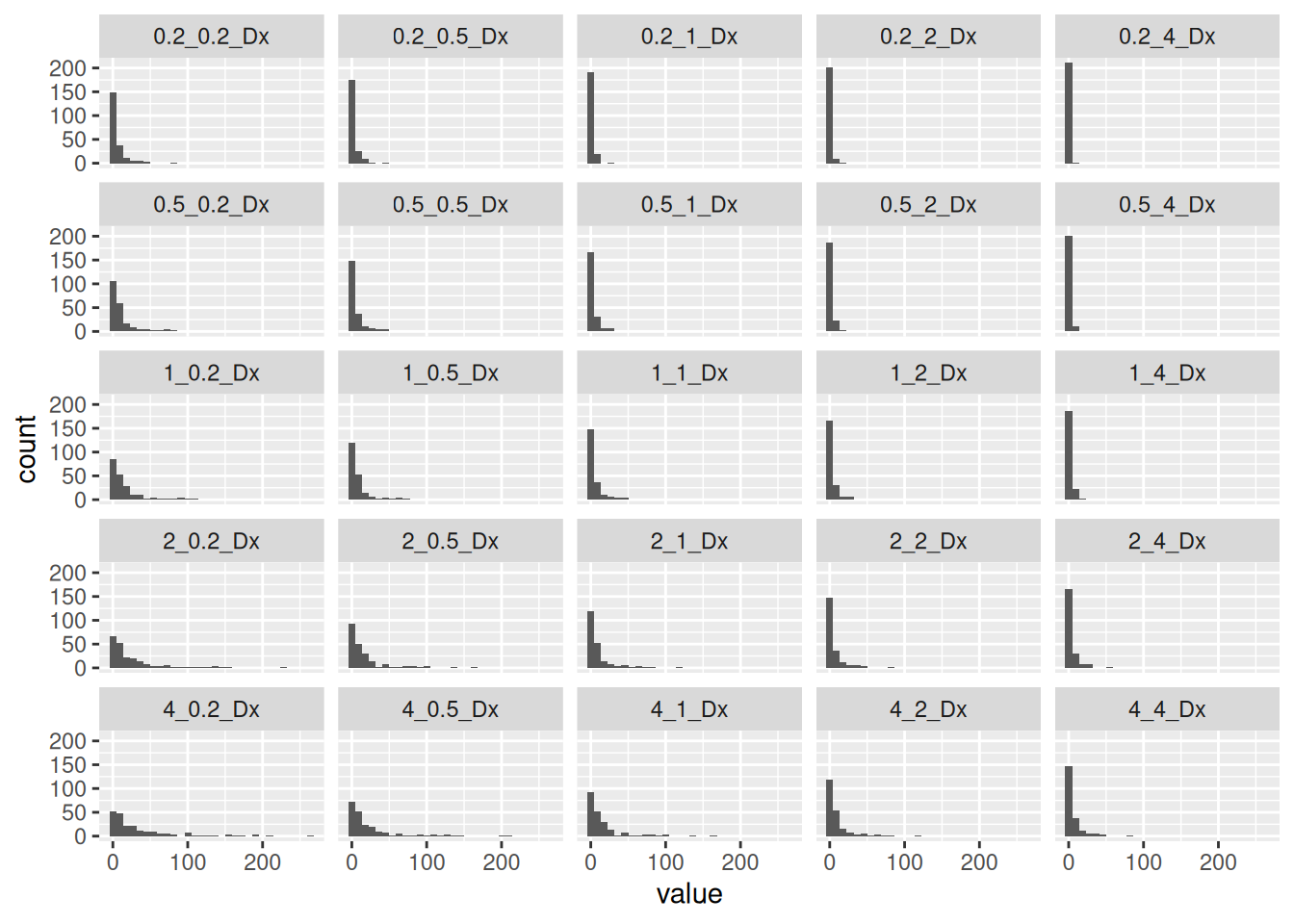
collect %>%
  select(ends_with("Dy")) %>%
  pivot_longer(cols=everything(), names_to="Name") %>%
  mutate(class=factor(Name)) %>%
  filter(value<300) %>%
  ggplot(aes(x=value)) +
    geom_histogram() +
    facet_wrap(~class)
collect %>%
  select(ends_with("Delta")) %>%
  pivot_longer(cols=everything(), names_to="Name") %>%
  mutate(class=factor(Name)) %>%
  filter(value<500) %>%
  ggplot(aes(x=value)) +
    geom_histogram() +
    facet_wrap(~class)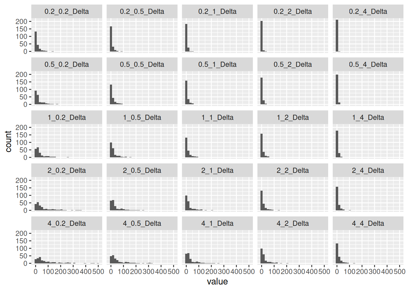
########   end testing

#   run it

df_kal <- df_utm3 %>%
  mutate(X=sf::st_coordinates(.)[,1],
         Y=sf::st_coordinates(.)[,2]) %>%
  sf::st_drop_geometry() %>%
  group_by(Date) %>%
    mutate(a=Kalman(X, Y, 4*Delta_dist/num, 0.5*New_dist)) %>%
    mutate(X2=a$X2,
           Y2=a$Y2) %>%
  ungroup()

df_kal <- df_kal %>%
  sf::st_drop_geometry() %>%
  sf::st_as_sf(coords=c("X2", "Y2"), crs=Seattle)

l2 <- df_kal %>%
  group_by(Date) %>%
  summarize(do_union=FALSE) %>%
  sf::st_cast("LINESTRING")

tmap::tmap_options(basemaps="OpenStreetMap")

tmap::tmap_mode("view") # set mode to interactive plots

tmap::tm_shape(l) +
  tmap::tm_lines() +
tmap::tm_shape(l2) +
  tmap::tm_lines(col="red") +
tmap::tm_shape(df_utm3 %>% select(Date, elevation, num, waypt)) +
  tmap::tm_dots(fill="red", size=0.5) +
tmap::tm_shape(df_kal %>% select(Date, elevation, num, waypt)) +
  tmap::tm_dots(fill="green", size=0.5)
Conclusion
I feel like I have a pretty robust process now for de-spiking and smoothing the coordinates, so the next step will be to do more radical things like gridding the data so that more interesting maps can be made.