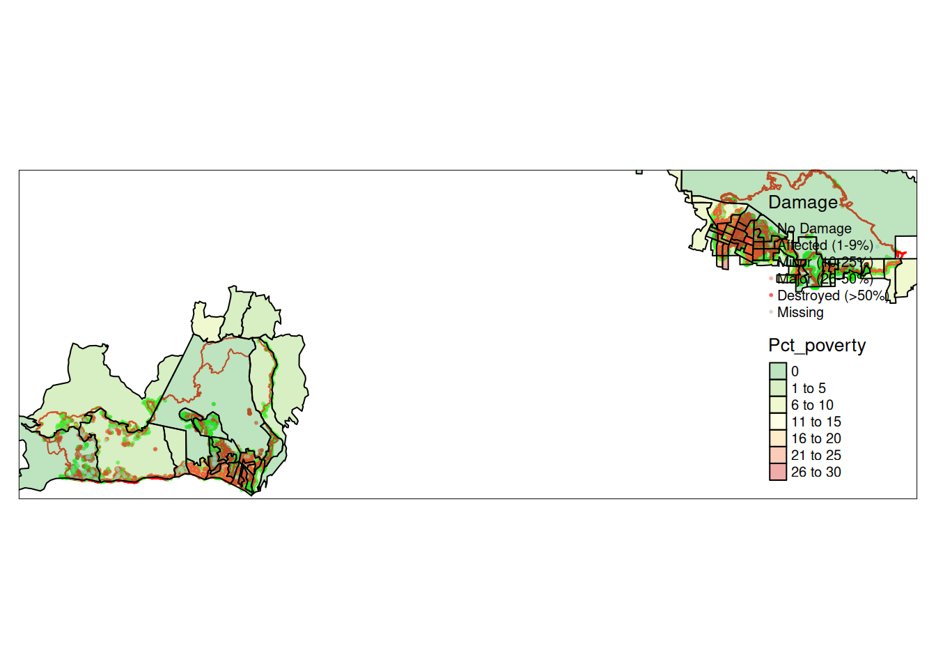
Developing a tool to overlay destruction with poverty levels
Author
Alan Jackson
Published
January 15, 2025
Mapping the LA fires and poverty levels
Yesterday I got an e-mail from a person at ERD (Episcopal Relief and Development) I have been working with. The question regarding the LA fires:
“Would it be relatively easy to show this damage data on a map with poverty levels?”
So I started trying to find the data. First I was able (with my primitive Arc skills) to create an Arcgis online map for the Eaton fire with the structure damage data overlain by poverty levels by census tract. I wasn’t able to do the same thing for the Palisades fire - I think the GIS author didn’t set the right permissions. With further searching I found the California Department of Forestry and Fire Protection data hub, where they have data for public download.
At first I downloaded the csv files, but I never could find documentation on what geoid and projection system they used for the coordinates, so I went back and downloaded the shapefiles. So in the rest of this, that is my starting point.
One advantage of having the data in my own hands, is that I can attach census block-groups to each point, so the resolution on where the poverty pockets are will be higher, and I can also generate statistics and plots quite easily.
library(tidyverse)
── Attaching core tidyverse packages ──────────────────────── tidyverse 2.0.0 ──
✔ dplyr     1.1.4     ✔ readr     2.1.5
✔ forcats   1.0.0     ✔ stringr   1.5.1
✔ ggplot2   3.5.1     ✔ tibble    3.2.1
✔ lubridate 1.9.4     ✔ tidyr     1.3.1
✔ purrr     1.0.2
── Conflicts ────────────────────────────────────────── tidyverse_conflicts() ──
✖ dplyr::filter() masks stats::filter()
✖ dplyr::lag()    masks stats::lag()
ℹ Use the conflicted package (<http://conflicted.r-lib.org/>) to force all conflicts to become errors
library(gt)library(tidycensus)library(sf)
Linking to GEOS 3.12.1, GDAL 3.8.4, PROJ 9.4.0; sf_use_s2() is TRUE
googlecrs <-"EPSG:4326"in_path <-"/home/ajackson/Dropbox/Rprojects/ERD/CA_Fire/Data/"path <-"/home/ajackson/Dropbox/Rprojects/ERD/CA_Fire/"# Read in the shapefiles we created to a simple featureEaton <-read_sf(paste0(in_path, "DINS_2025_Eaton_Public_View/","DINS_2025_Eaton_Public_View.shp"))summary(Eaton) # check to see what it looks like. Could also do plot(temp)
    OBJECTID       GLOBALID            DAMAGE           STRUCTURET
 Min.   :    1   Length:18421       Length:18421       Length:18421
 1st Qu.: 4657   Class :character   Class :character   Class :character
 Median : 9302   Mode  :character   Mode  :character   Mode  :character
 Mean   : 9308
 3rd Qu.:13953
 Max.   :18620
          geometry
 POINT        :18421
 epsg:3857    :    0
 +proj=merc...:    0
Eaton <- Eaton %>%mutate(Fire="Eaton") %>%st_transform(googlecrs) # get to a better geoid compatible with Open maps# Create a tiny date file with the date for that fileMydate <-file.info(paste0(in_path, "DINS_2025_Eaton_Public_View/","DINS_2025_Eaton_Public_View.shp")) %>%select(ctime)Mydate <-as.character(lubridate::as_date(Mydate$ctime))saveRDS(Mydate, paste0(path, "Date_string.rds"))Palisades <-read_sf(paste0(in_path, "DINS_2025_Palisades_Public_View/","DINS_2025_Palisades_Public_View.shp"))summary(Palisades) # check to see what it looks like. Could also do plot(temp)
    OBJECTID       GLOBALID            DAMAGE           STRUCTURET
 Min.   :    1   Length:12040       Length:12040       Length:12040
 1st Qu.: 3824   Class :character   Class :character   Class :character
 Median : 6960   Mode  :character   Mode  :character   Mode  :character
 Mean   : 6869
 3rd Qu.:10047
 Max.   :13438
          geometry
 POINT        :12040
 epsg:3857    :    0
 +proj=merc...:    0
Palisades <- Palisades %>%mutate(Fire="Palisades") %>%st_transform(googlecrs)# Read in fire perimetersPerimeters <-read_sf(paste0(in_path, "CA_Perimeters_NIFC_FIRIS_public_view/","CA_Perimeters_NIFC_FIRIS_public_view.shp")) %>%filter(stringr::str_detect(incident_n, "Eaton|PALISADES")) %>%st_transform(googlecrs) %>%st_make_valid()summary(Perimeters)
    OBJECTID      GlobalID             type              source
 Min.   :1279   Length:6           Length:6           Length:6
 1st Qu.:1289   Class :character   Class :character   Class :character
 Median :1296   Mode  :character   Mode  :character   Mode  :character
 Mean   :1293
 3rd Qu.:1298
 Max.   :1300

   poly_DateC           mission           incident_n         incident_1
 Min.   :2025-01-08   Length:6           Length:6           Length:6
 1st Qu.:2025-01-10   Class :character   Class :character   Class :character
 Median :2025-01-11   Mode  :character   Mode  :character   Mode  :character
 Mean   :2025-01-10
 3rd Qu.:2025-01-12
 Max.   :2025-01-12
 NA's   :1
   area_acres     descriptio          FireDiscov           CreationDa
 Min.   :13299   Length:6           Min.   :2025-01-07   Min.   :2025-01-08
 1st Qu.:13995   Class :character   1st Qu.:2025-01-07   1st Qu.:2025-01-10
 Median :14013   Mode  :character   Median :2025-01-07   Median :2025-01-13
 Mean   :16723                      Mean   :2025-01-07   Mean   :2025-01-13
 3rd Qu.:19493                      3rd Qu.:2025-01-07   3rd Qu.:2025-01-15
 Max.   :23707                      Max.   :2025-01-08   Max.   :2025-01-18
                                    NA's   :4            NA's   :4
    EditDate           displaySta                 geometry
 Min.   :2025-01-11   Length:6           MULTIPOLYGON :6
 1st Qu.:2025-01-13   Class :character   epsg:4326    :0
 Median :2025-01-16   Mode  :character   +proj=long...:0
 Mean   :2025-01-16
 3rd Qu.:2025-01-18
 Max.   :2025-01-21
 NA's   :4
Functions
options(tigris_use_cache =TRUE)# Retrieve the census dataget_ACS <-function(State, County) {# Now let's prepare the block-group data acs_vars <-c(Pop="B01001_001", # ACS population estimateMed_inc="B19013_001", # median household income, blk grpPer_cap_inc="B19301_001", # Per capita income, blk grpFam="B17010_001", # Families, blk grpFam_in_poverty="B17010_002", # Families in poverty, blk grpAggreg_inc="B19025_001", # Aggregate household income, blk grpHouseholds="B11012_001", # Households, blk grpMed_age="B01002_001") # median age, blk grp ACS <-get_acs(geography="block group",variables=acs_vars,year=2020,county=County,state=State,output="wide",geometry=TRUE) ACS <- ACS %>%mutate(Pct_poverty=as.integer(signif(100*Fam_in_povertyE/FamE, 0))) %>%select(GEOID, Pop_acs=PopE, Med_inc=Med_incE, Per_cap_in=Per_cap_incE,Fam=FamE, Fam_in_poverty=Fam_in_povertyE, Aggreg_inc=Aggreg_incE, Pct_poverty, Households=HouseholdsE, Med_ageE=Med_ageE) ACS <- sf::st_transform(ACS, googlecrs) %>%# get to a common geoid sf::st_make_valid()return(ACS)}
Clean up fire data
The fire data has a weird text field for the damage level:
So for it to be useful in analysis, I need to turn it into a factor.
Similarly, the field describing the structure type should also be a factor.
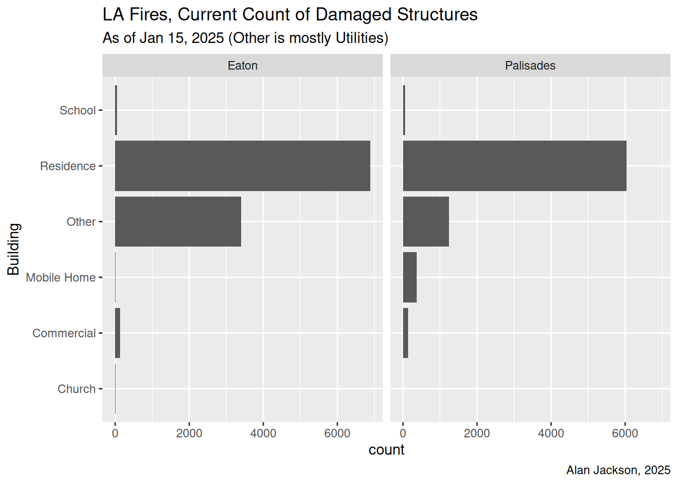
In some ways it has too much detail (“Single Family Residence Multi Story”, “Single Family Residence Single Story”), so I will also create a new variable to collapse the categories of buildings to residences, businesses, and other.
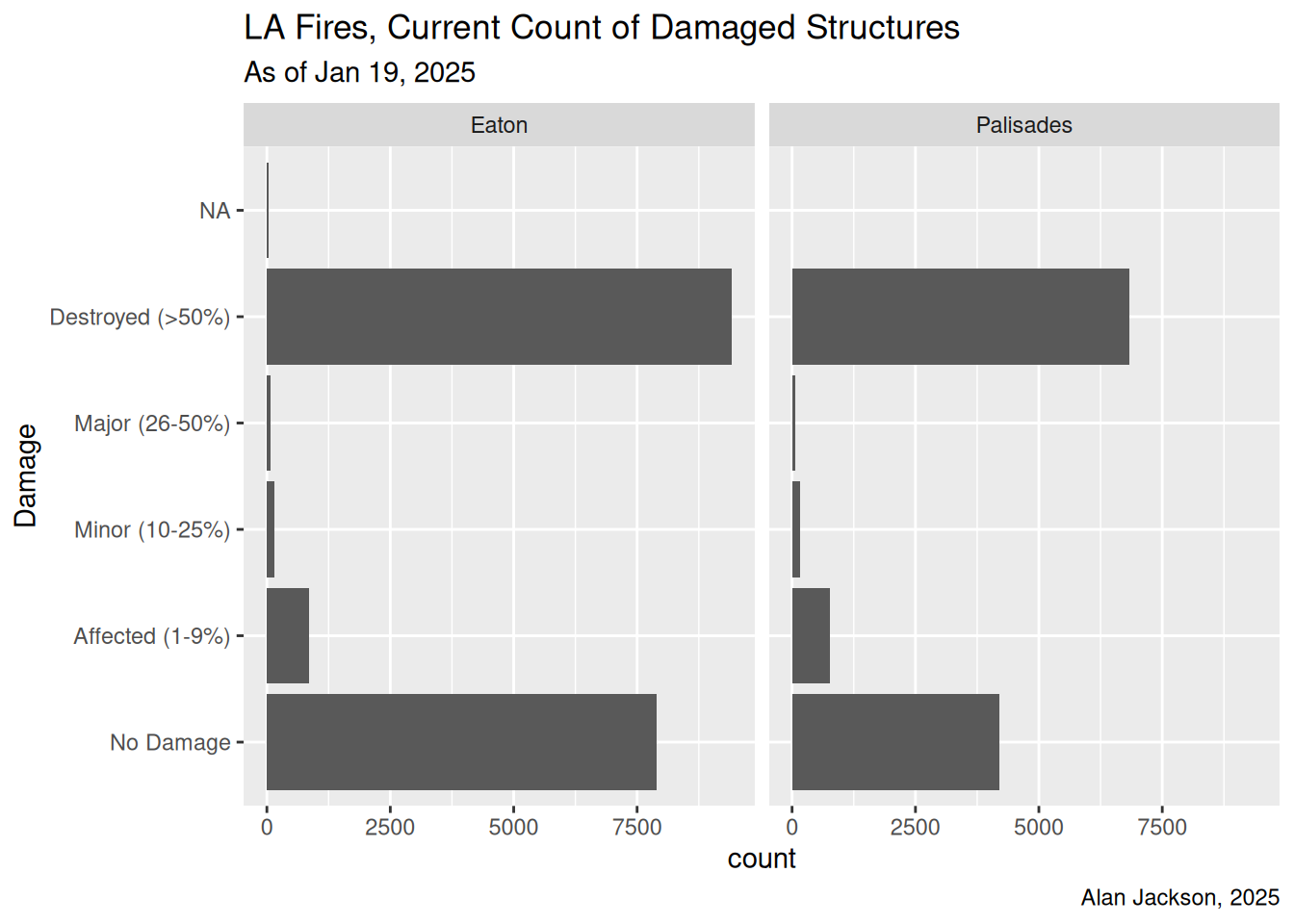
df %>%ggplot(aes(x=Damage)) +geom_bar() +facet_wrap(~Fire) +coord_flip() +labs(title="LA Fires, Current Count of Damaged Structures",subtitle="As of Jan 19, 2025 ",caption="Alan Jackson, 2025")
# This gets run the first time and then saved# Census <- get_ACS('CA', "Los Angeles") %>% # replace_na(list(Pct_poverty=0)) %>% # filter(Pop_acs>0)# Read in saved census dataCensus <-readRDS(paste0(path, "Census.rds")) # already saved# Extract block groups that intersect the fire perimeter polygonCensus <- Census[Perimeters,]