Analyse Sea Level Data from UCS

The Union of Concerned Scientists developed a spreadsheet of chronically inundated propeties by zipcode, climate scenario, and year. In this exercise we will try to identify the most vulnerable properties based on flood danger and average income.

The data we are working with here looks at chronic inundation (flooding at least 26 times per year), usually high-tide flooding.

library(tidyverse)
library(stringr)
library(tmap)
library(tigris)

us_geo <- tigris::states(class = "sf", progress_bar = FALSE) 

googlecrs <- "EPSG:4326"

path <- "/home/ajackson/Dropbox/Rprojects/TexasDioceseCreationCare/Data/"
output_path <- "/home/ajackson/Dropbox/projects/CeationCareTaskforce/"
Curated_path <- "/home/ajackson/Dropbox/Rprojects/Curated_Data_Files/"

df <- readRDS(paste0(Curated_path, "SeaLevel/UCS_spreadsheet.rds"))

Let’s look at the highest risk zipcodes

We’ll look at absolute numbers of people at risk, as well as the largest proportion at risk. We’ll restrict ourselves to the two nearer-term scenarios, “2030 High” and “2035 Intermediate”

#   filter down to what is interesting

df <- df %>%  
  # filter(str_detect(sheet, "2030 High|2035 Intermediate")) %>% 
  select(sheet, Year, State, Zip=`ZIP Code`, Homes_Risk=`Homes at Risk`,
         Pop_at_risk=`Population currently housed in at risk homes`,
         Total_Homes=`Total Homes`, Total_Pop=`Total Population`) %>% 
  mutate(Homes_ratio=signif(100*Homes_Risk/Total_Homes, 3),
         Pop_ratio=signif(100*Pop_at_risk/Total_Pop, 3)) %>% 
  filter(Total_Homes>100) %>% 
  filter(Total_Pop>100) %>% 
  mutate(Zip=as.character(Zip))

Let’s get some census data by zipcode to attach to the data

v20 <- tidycensus::load_variables(2020, "acs5", cache = TRUE)

# B19013_001 MEDIAN HOUSEHOLD INCOME IN THE PAST 12 MONTHS (IN 2020 INFLATION-ADJUSTED DOLLARS)
# B17025_001 POVERTY STATUS IN THE PAST 12 MONTHS BY NATIVITY
# B19001_001 HOUSEHOLD INCOME IN THE PAST 12 MONTHS (IN 2020 INFLATION-ADJUSTED DOLLARS)
# B19025_001 AGGREGATE HOUSEHOLD INCOME IN THE PAST 12 MONTHS (IN 2020 INFLATION-ADJUSTED DOLLARS)
# B01003_001 TOTAL POPULATION

foo <- tidycensus::get_acs(geography = "zcta", #    Zip Code Tabulation Area
                variables = c("B19013_001", "B17025_002", "B19001_001", 
                              "B19025_001", "B01003_001"), 
                year = 2020, geometry=FALSE)

#   I'll merge the polygons in later

ZCTA_geom <- tidycensus::get_acs(geography = "zcta",
                variables =  "B01003_001", 
                progress_bar = FALSE,
                year = 2020, geometry=TRUE)

foobar <- foo %>% 
  select(GEOID, variable, estimate) %>% 
  pivot_wider(id_cols=GEOID, names_from=variable, values_from=estimate) %>% 
  rename(Zip=1, Med_income=2, In_Poverty=3, House_Income=4, Total_income=5,
         Total_Pop_acs=6)

Let’s do a join

foo <- df %>% 
  left_join(., foobar, by="Zip")

Some cleanup

foo <- foo %>% 
  filter(Homes_Risk>100) %>% 
  filter(Total_Pop_acs>100) %>% 
  mutate(Avg_income=Total_income/Total_Pop_acs) %>% 
  mutate(Poverty_pct=signif(100*In_Poverty/Total_Pop_acs, 3))

#   Save for later

saveRDS(foo, paste0(Curated_path,"SeaLevel/UCS_data.rds"))

Make maps

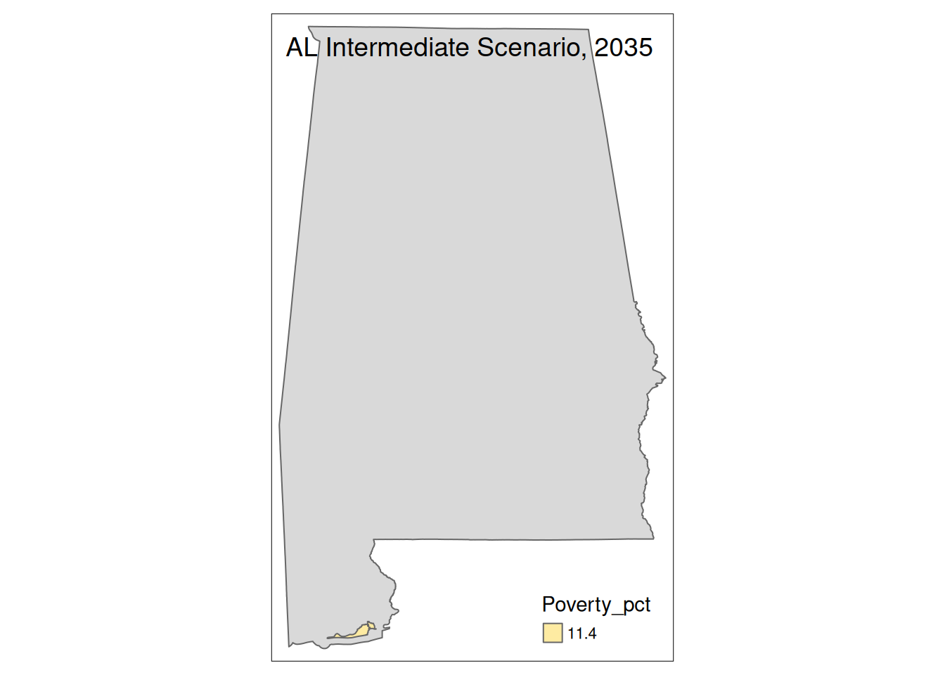
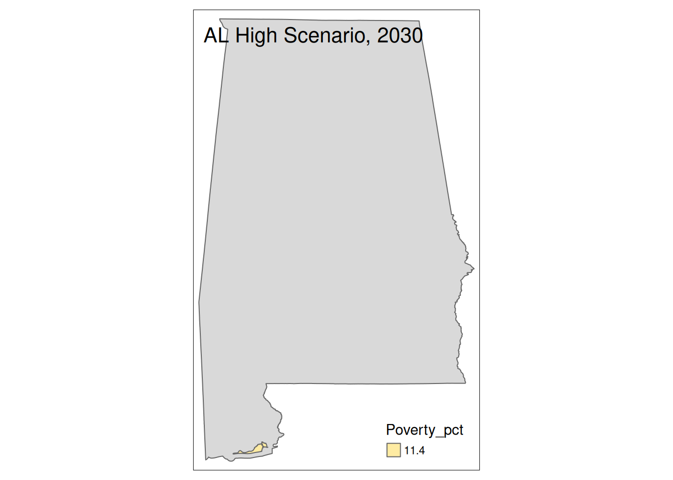
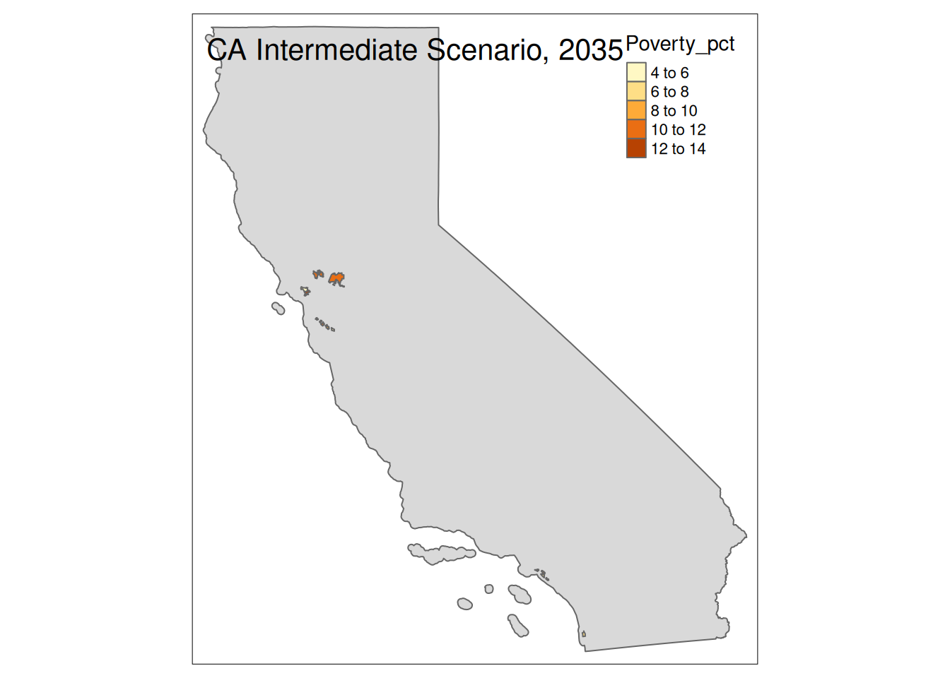
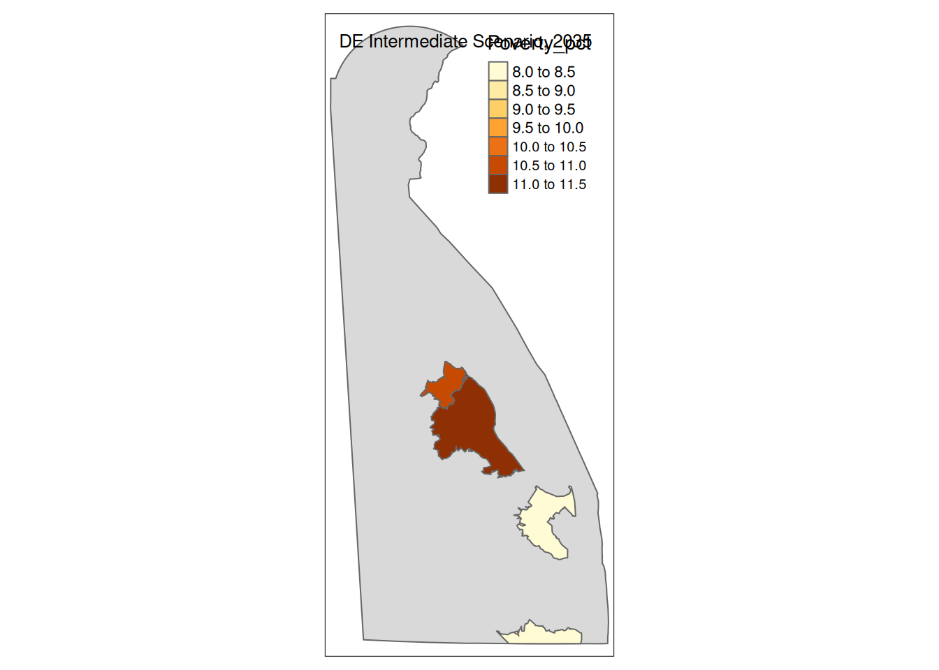
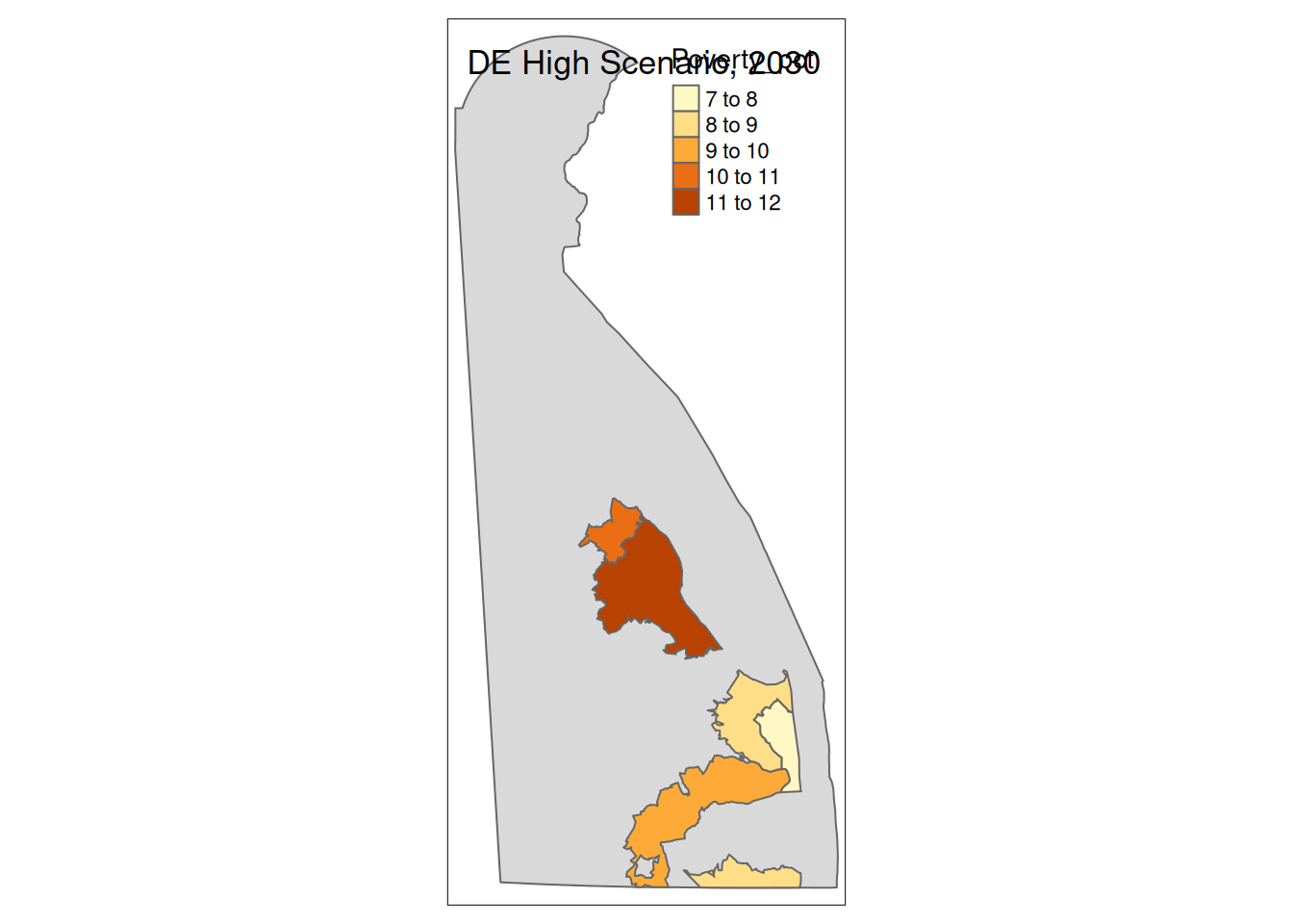
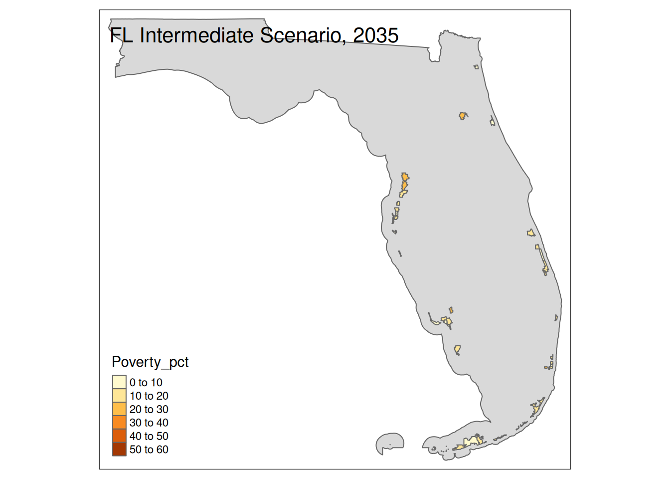
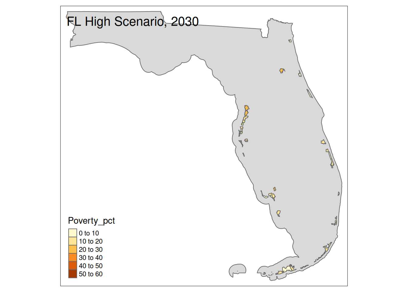
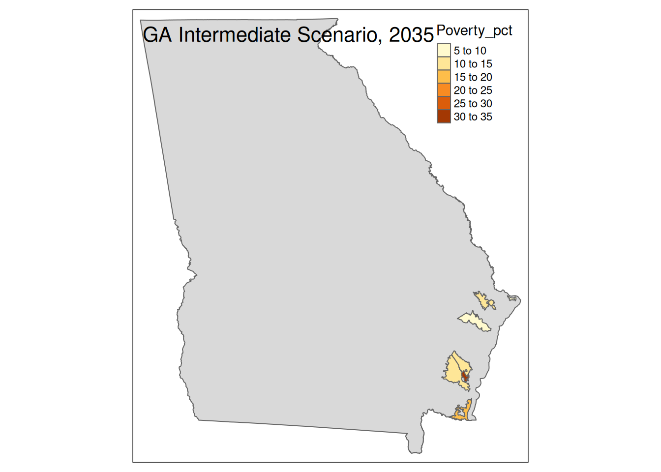
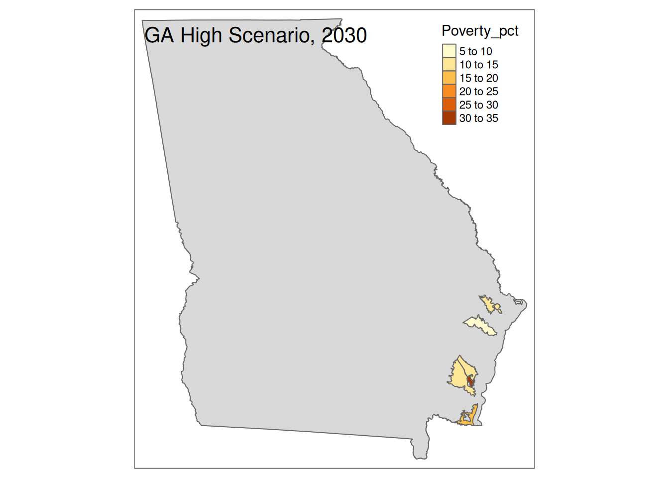
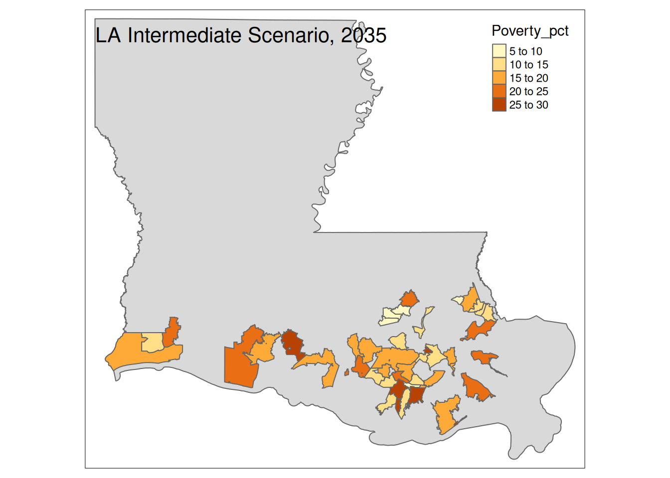
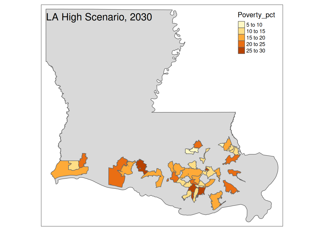
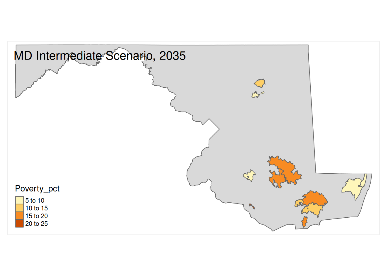
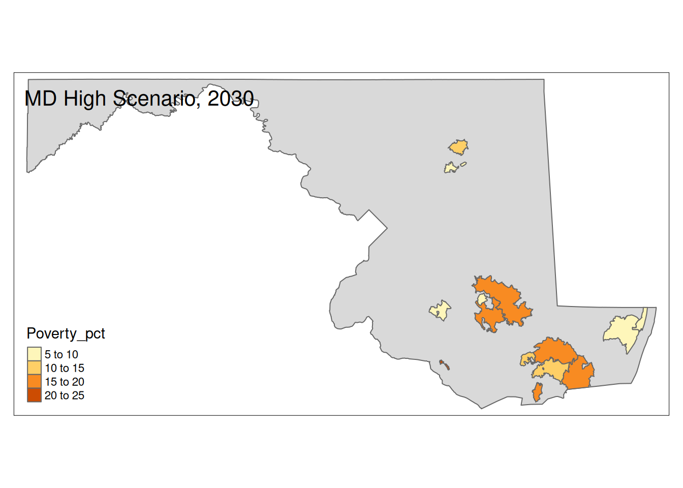
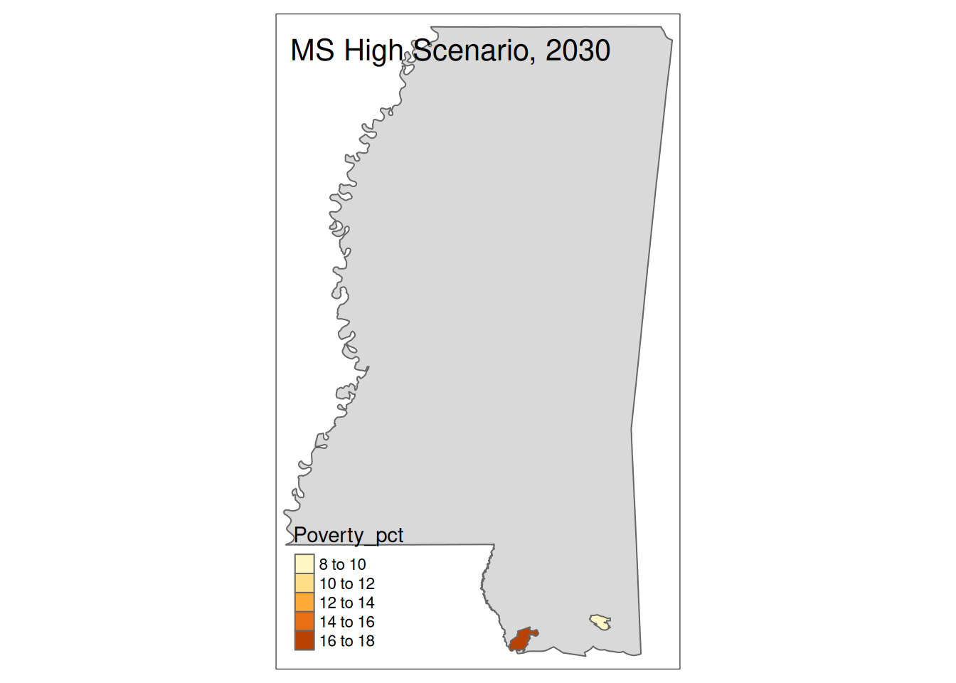
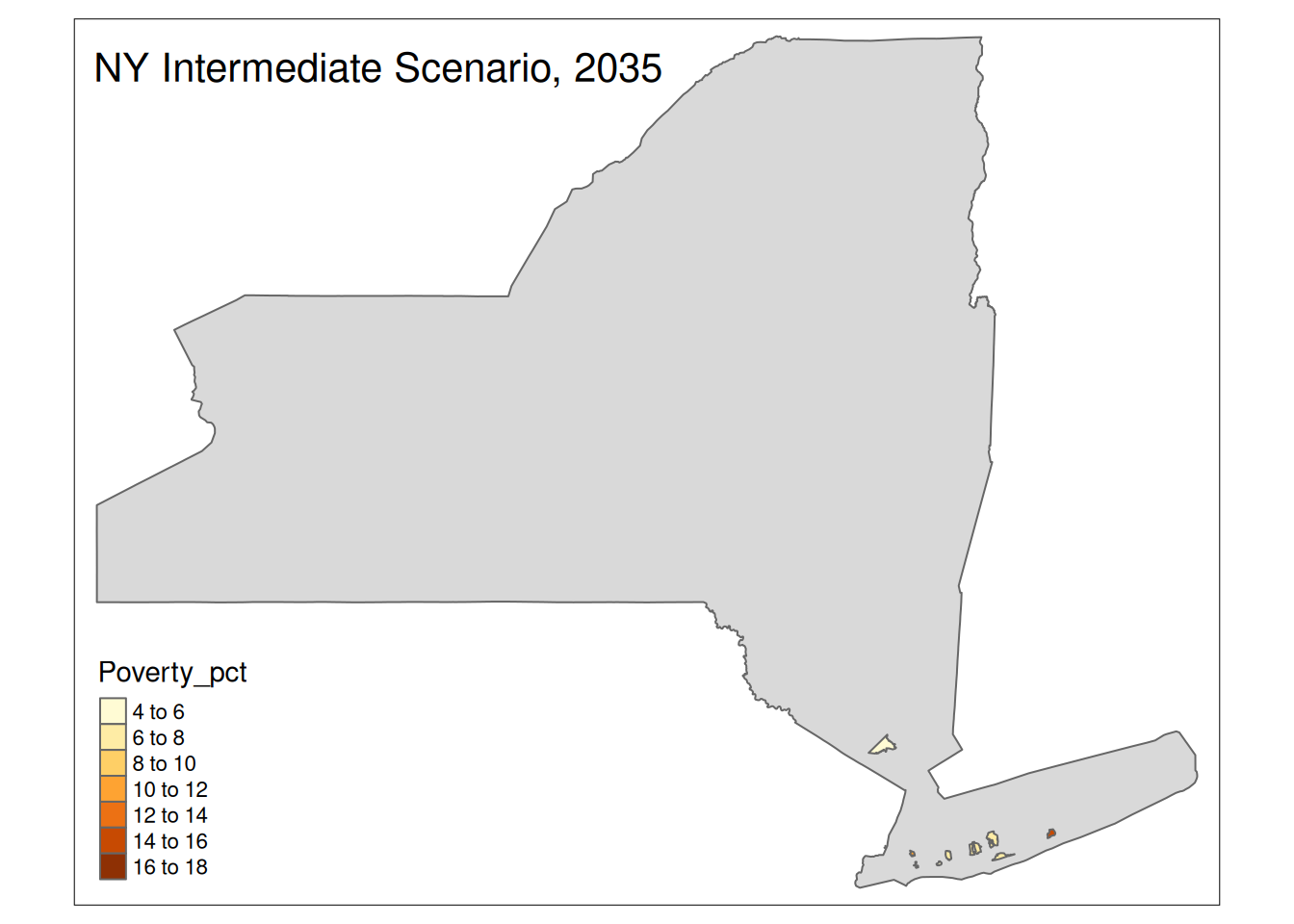
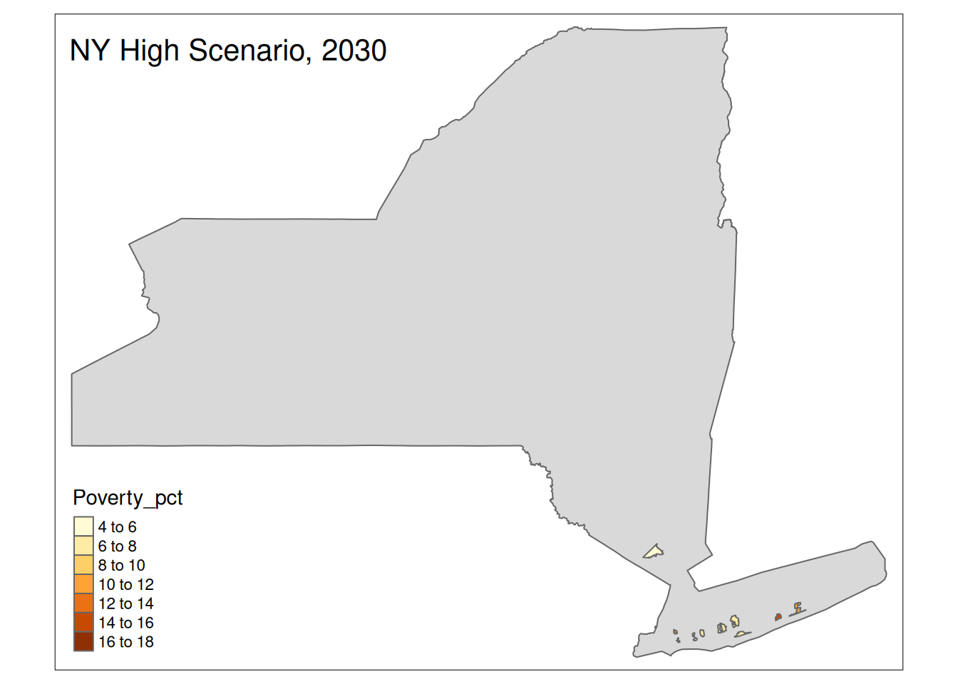
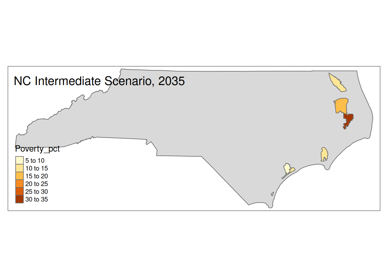
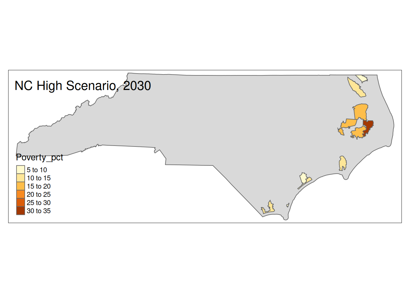
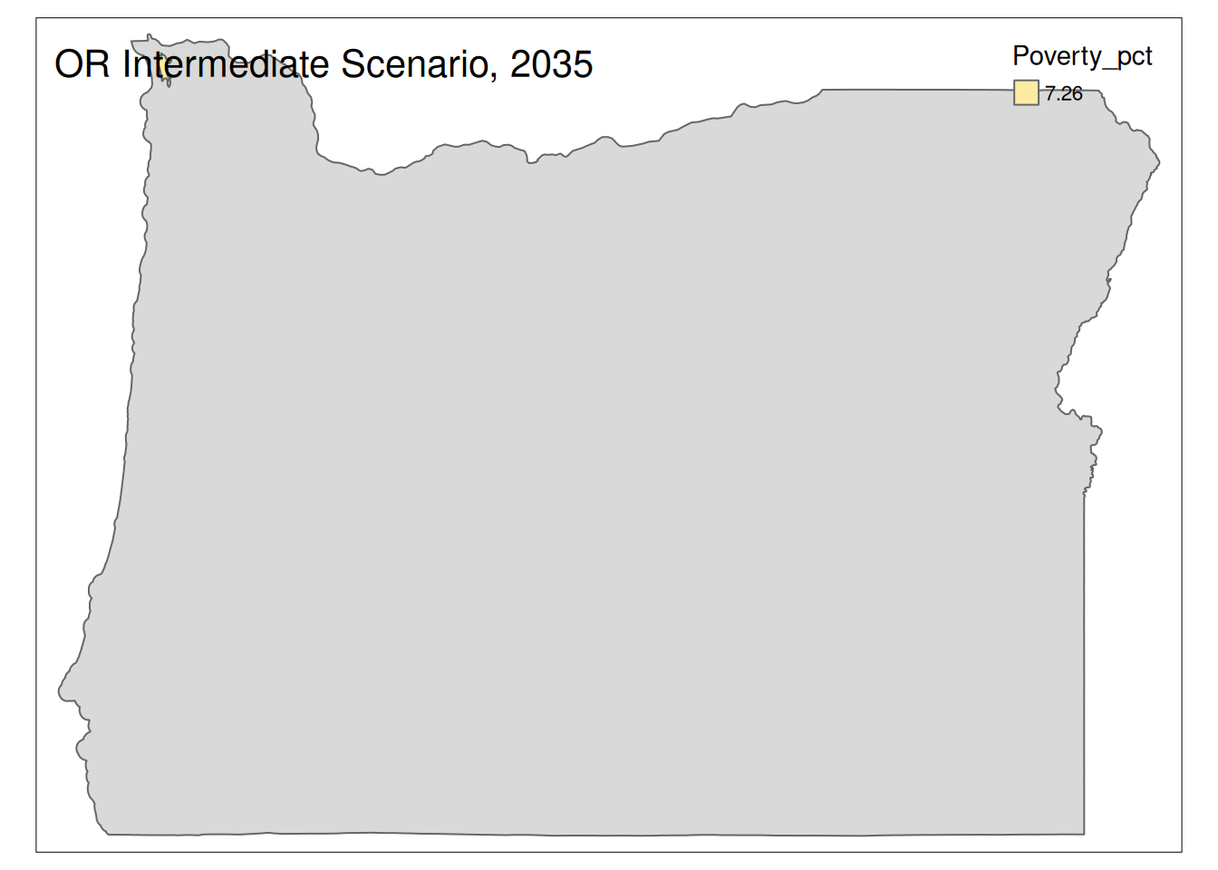
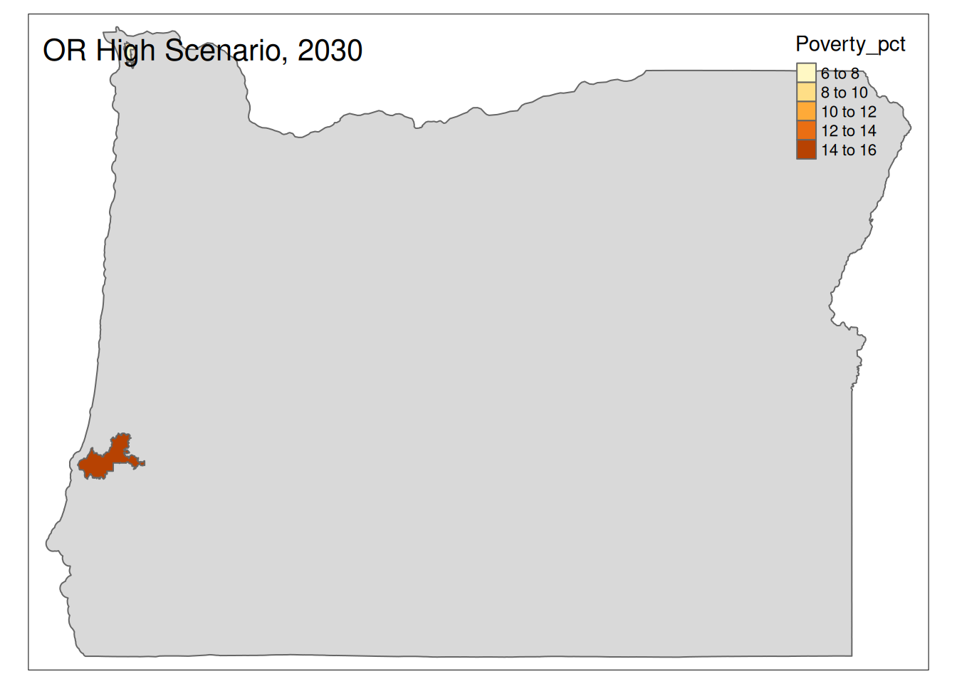
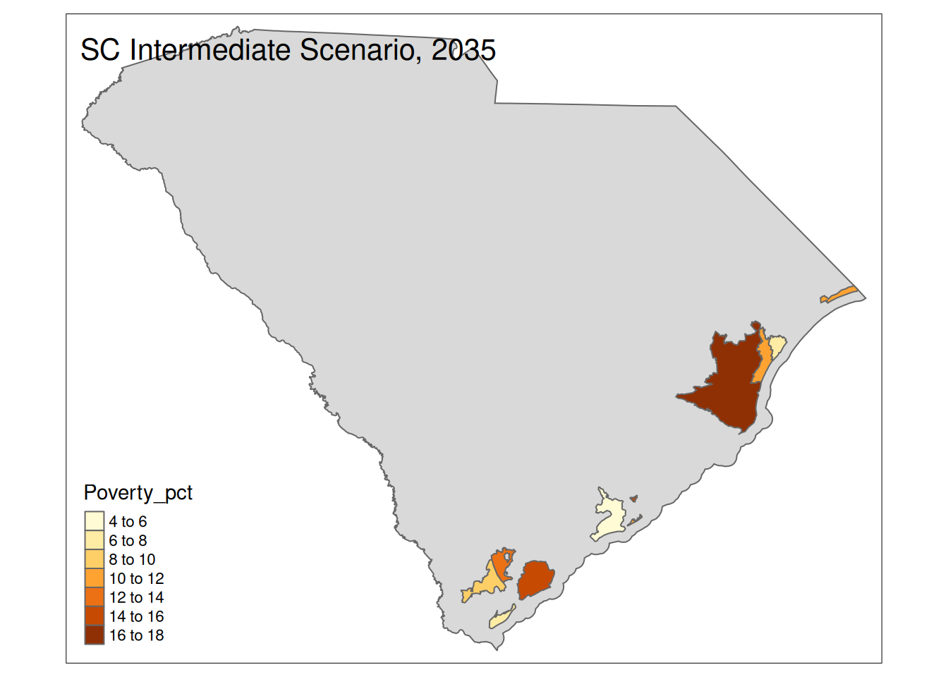
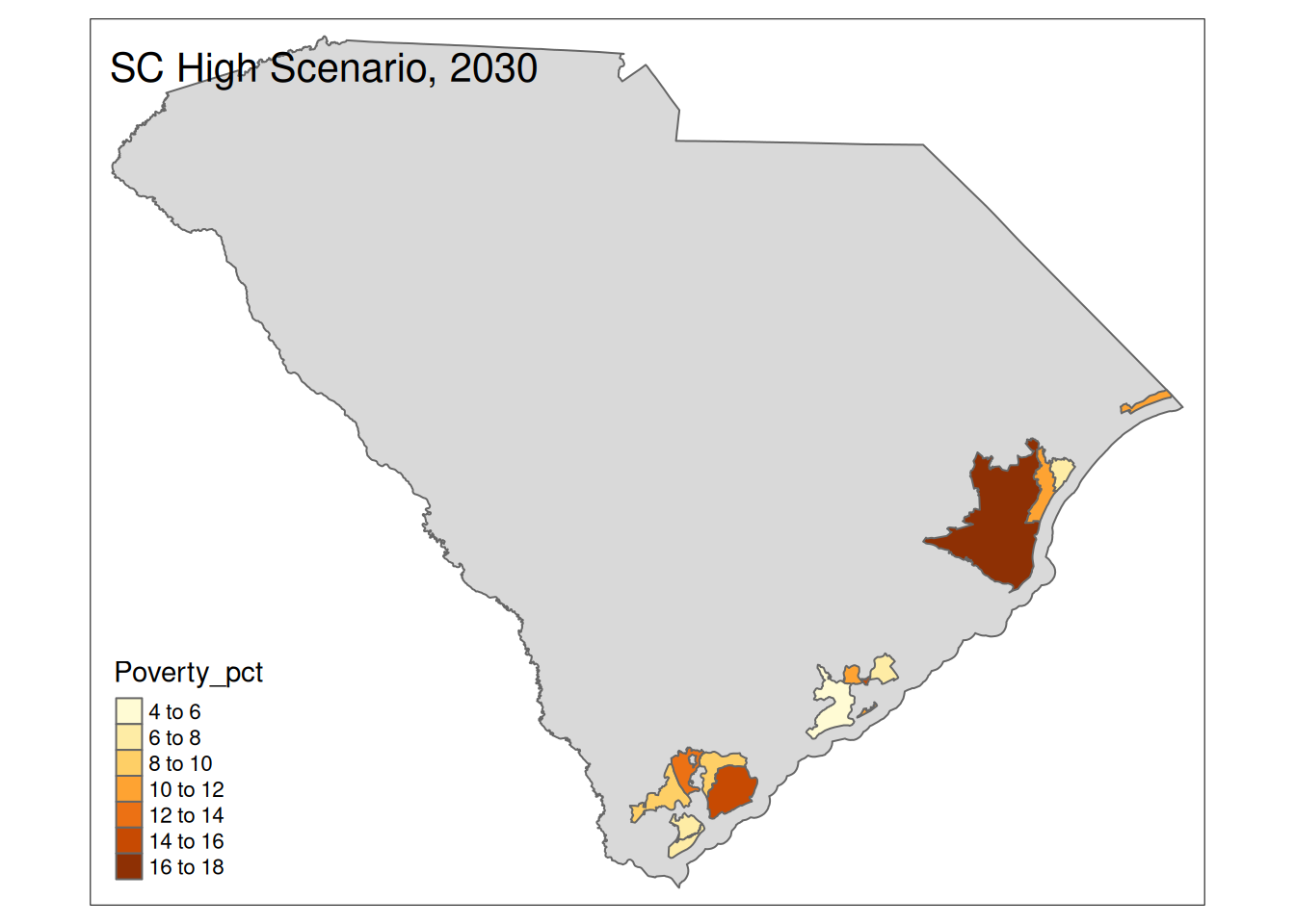
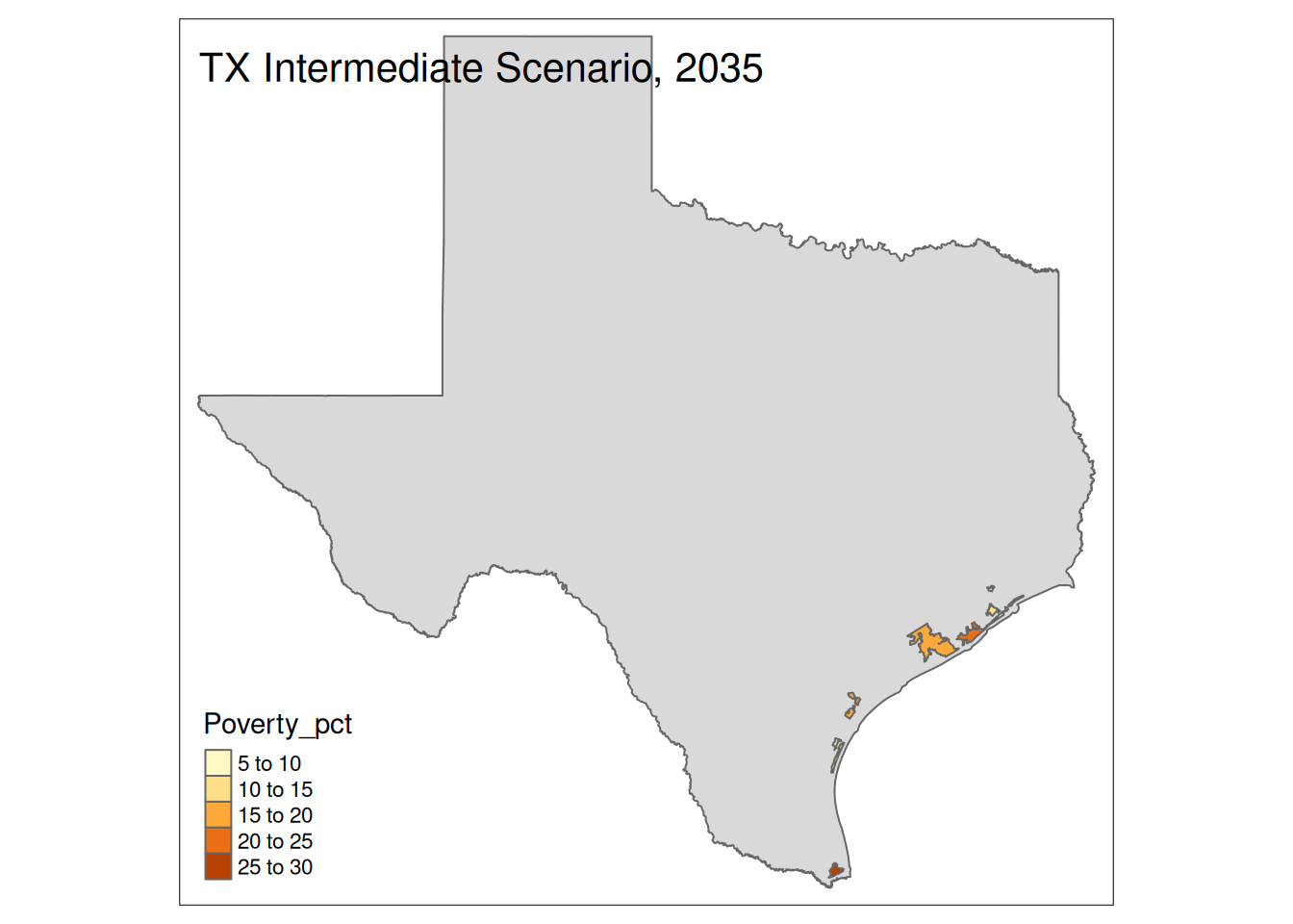
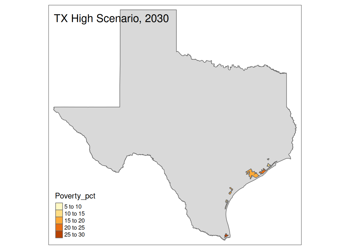
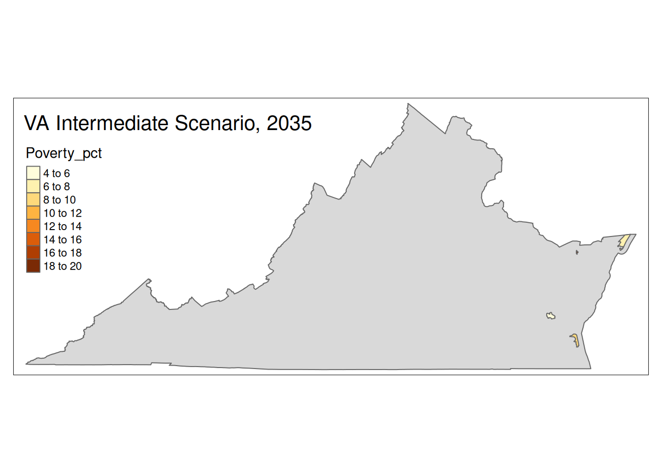
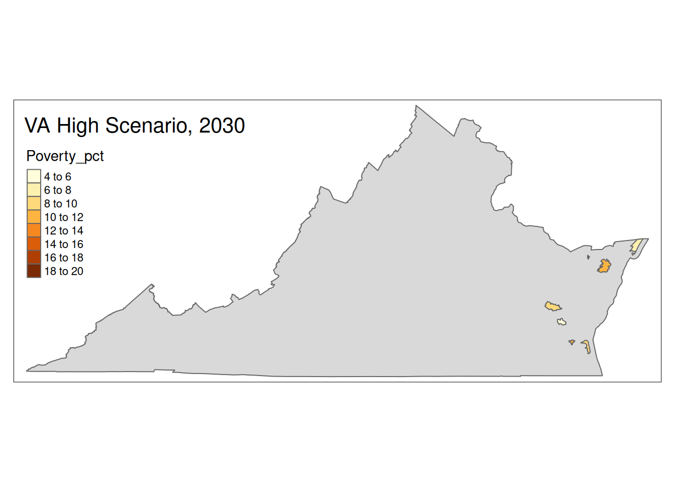
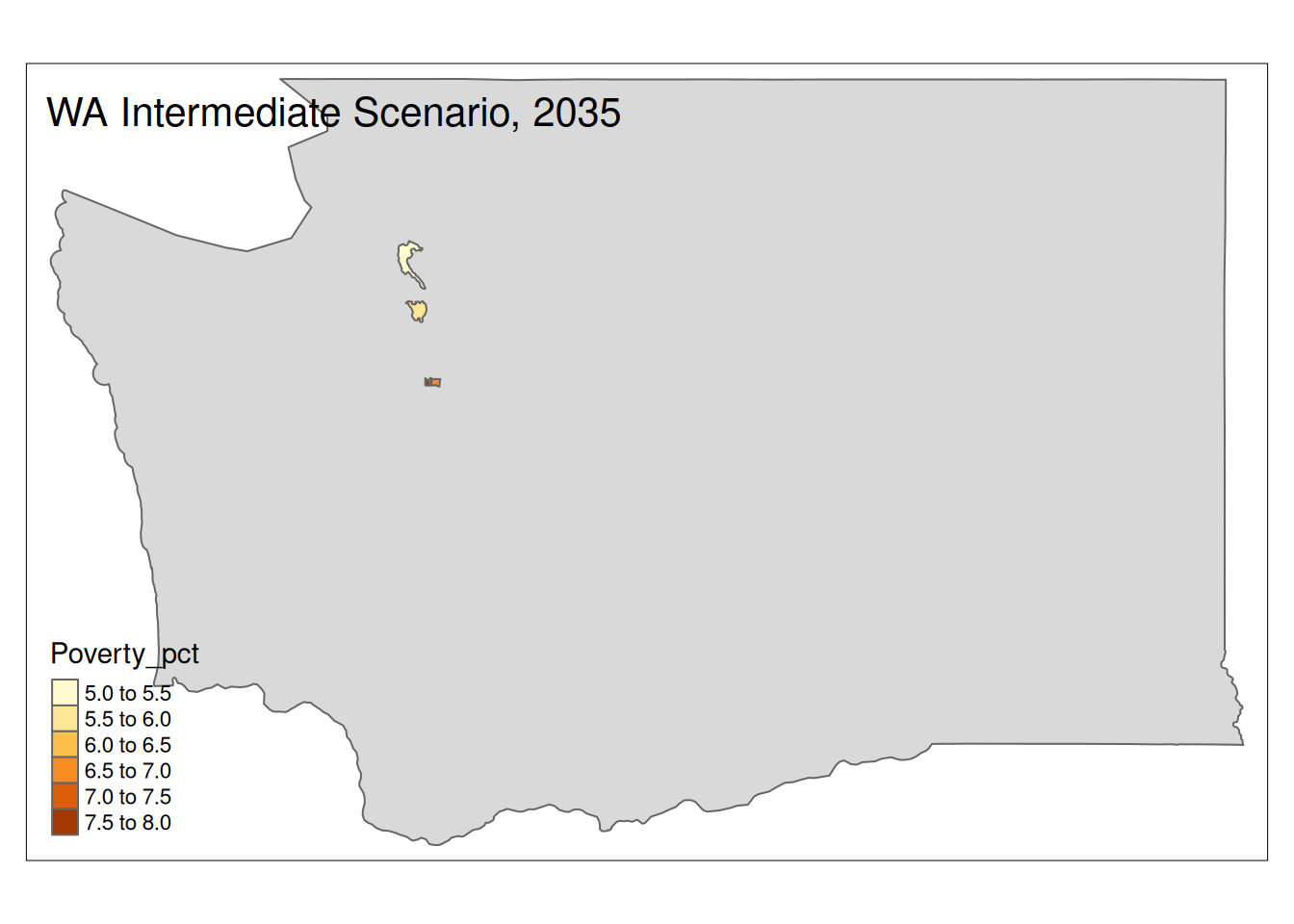
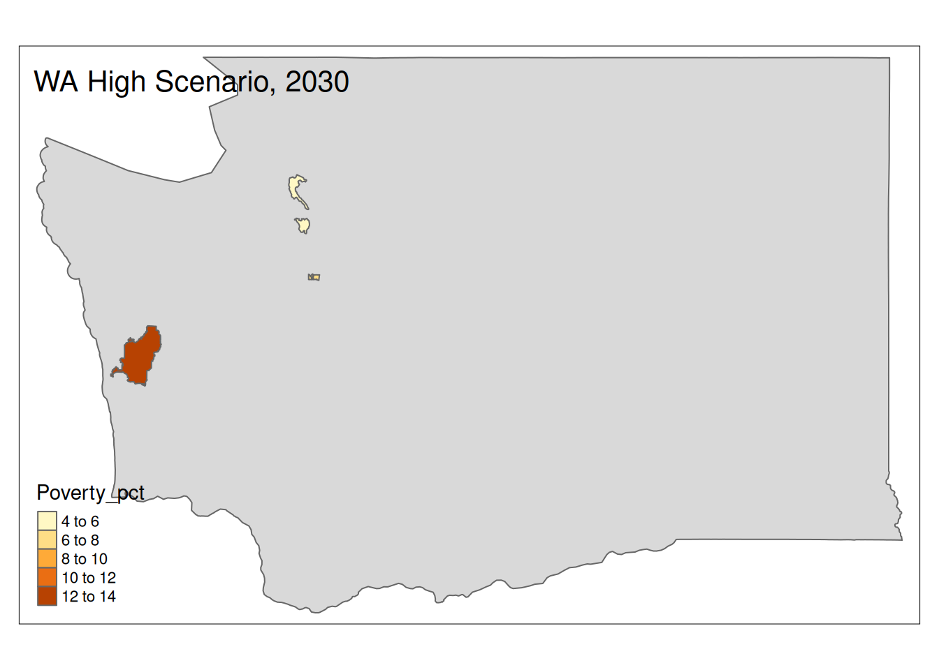
Two maps, 2030 High and 2035 Intermediate scenarios, color by pct in poverty.

Popup data for each zip code are the zip code, the number of homes at risk, and the ratio of homes at risk divided by total homes.

#   first an interactive map for QC

#   Add the geometry

foo2 <- left_join(foo, ZCTA_geom, by=join_by(Zip==GEOID)) %>% 
  select(-NAME, -variable, -estimate, -moe) %>% 
  filter(Poverty_pct>5) %>% 
  mutate(Poverty_pct=signif(Poverty_pct, 3)) %>% 
  sf::st_as_sf()
#   Save for later

saveRDS(foo2, paste0(Curated_path,"SeaLevel/UCS_sfdata.rds"))

High30 <- foo2 %>% filter(str_detect(sheet, "2030"))
Inter35 <- foo2 %>% filter(str_detect(sheet, "2035"))

#   map
tmap::tmap_options(basemaps="OpenStreetMap")
tmap_mode("view")

tm_shape(Inter35) +
  tm_polygons("Poverty_pct", alpha=0.5, popup.vars=c("Zip", 
                                                     "Homes_Risk",
                                                     "Homes_ratio")) +
  tm_dots(size=0.02) +
tm_shape(High30) +
  tm_polygons("Poverty_pct", alpha=0.5, popup.vars=c("Zip", "Homes_Risk",
                                                     "Homes_ratio")) 

#   do maps by state

tmap_mode("plot")
data("World")
for (state in unique(foo2$State)) {
  State <- us_geo %>% filter(str_detect(STUSPS, state))
  
  if (nrow(Inter35 %>% sf::st_drop_geometry() %>%  filter(State==state))>0){
  
    plot <- 
            tm_shape(State) +
              tm_polygons() +
            tm_shape(Inter35 %>% filter(State==state)) +
              tm_polygons("Poverty_pct") +
            tm_layout(title=paste(state, "Intermediate Scenario, 2035"))
    
    print(plot)
  }
  
  if (nrow(High30 %>% sf::st_drop_geometry() %>%  filter(State==state))>0){
    plot <- 
            tm_shape(State) +
              tm_polygons() +
            tm_shape(High30 %>% filter(State==state)) +
              tm_polygons("Poverty_pct") +
            tm_layout(title=paste(state, "High Scenario, 2030"))
    
    print(plot)
  }
  
}