library(tidyverse)
library(stars)
library(terra)
library(tidyterra)
googlecrs <- "EPSG:4326"
localUTM <- "EPSG:32615"
inputcrs <- "EPSG:4269" # from metadata file
path <- "/home/ajackson/Dropbox/Rprojects/TexasDioceseCreationCare/Data/"
# Church locations
Parishes <- readRDS(paste0(path, "Parishes.rds"))
# Define an AOI
bbox <- sf::st_bbox(sf::st_transform(Parishes, crs=inputcrs))
bbox["xmin"] <- -96.38
bbox["xmax"] <- -93.66
bbox["ymin"] <- 28.39
bbox["ymax"] <- 30.47
# Expand box by 20% to give a little extra room
expand_box <- function(bbox, pct=0.2){
Dx <- (bbox[["xmax"]]-bbox[["xmin"]])*pct
Dy <- (bbox[["ymax"]]-bbox[["ymin"]])*pct
bbox["xmin"] <- bbox["xmin"] - Dx
bbox["xmax"] <- bbox["xmax"] + Dx
bbox["ymin"] <- bbox["ymin"] - Dy
bbox["ymax"] <- bbox["ymax"] + Dy
return(bbox)
}
Basemap_attribution <- 'attribution: © <a href="https://www.openstreetmap.org/copyright">OpenStreetMap</a> contributors'Read Storm Surge data
Mapping
Texas
Disasters
Diocesan Taskforce
Using NOAA storm surge grids to predict maximum surge at numerous locations.
Setup
Data downloaded from https://www.nhc.noaa.gov/nationalsurge/
Zachry, B. C., W. J. Booth, J. R. Rhome, and T. M. Sharon, 2015: A National View of Storm Surge Risk and Inundation. Weather, Climate, and Society, 7(2), 109–117. DOI: http://dx.doi.org/10.1175/WCAS–D–14–00049.1
- Data comes in NAD83
Each dataset contains an ESRI World File (.tfw) and metadata .xml file. These GeoTIFFs are 8-bit unsigned integer raster datasets that correspond to 1 ft inundation bins (e.g., Class Value 1 corresponds to the 0-1 ft inundation bin, Class Value 2 corresponds to the 1-2 ft inundation bin, and so on). The maximum Class Value is 21, and inundation in excess of 20 ft is assigned a Class Value of 21. A Class Value of 99 is assigned to leveed areas. A more detailed description of the data can be found in the associated metadata.
Read in the files and clip to AOI
Read in Cat 3 data and use the data extent to build a box.
Do a little test using one church to see what a 100 meter circle looks like.
Plot the rasters, and then make a nice map showing affected churches and the depth of storm surge.
x <- terra::rast(paste0(path, "US_SLOSH_MOM_Inundation_v3/us_Category3_MOM_Inundation_HIGH.tif"))

#   Clip to AOI

cropped <- terra::crop(x, bbox)
|---------|---------|---------|---------|
=========================================
#   The data has holes in it and I really don't want to take the depth
#   at a single point - better would be to average water depth for
#   about a block around the church, 100 meters say. Let's see what
#   that looks like

 pt1 <- sf::st_transform(Parishes, crs=inputcrs)[Parishes$Label=="Saint Augustine of Hippo",] %>%
   st_buffer(100) %>% st_as_sf() # Units are meters

# Add ID number to Parishes
Parishes <- Parishes %>%
  mutate(ID=row_number())

#   pts are really polygons surrounding church locations
pts <- sf::st_transform(Parishes, crs=inputcrs) %>%
  st_buffer(100) %>% st_as_sf() # Units are meters

 pt <- sf::st_transform(Parishes, crs=inputcrs)[Parishes$Label=="Saint Augustine of Hippo",]

 box <- sf::st_transform(Parishes, crs=inputcrs)[Parishes$Label=="Saint Augustine of Hippo",] %>%
   st_buffer(1200) %>% st_as_sf() %>% st_bbox()


 Base_basemapR <- basemapR::base_map(box, basemap="mapnik", increase_zoom=5)

 pt1 %>%
   ggplot() +
   Base_basemapR +
   geom_sf(aes(alpha=0.4))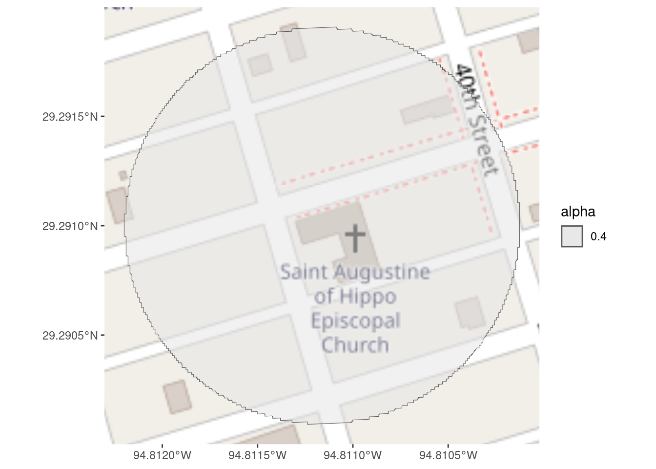
ggplot() +
  geom_spatraster(data=cropped) +
  geom_sf(data=sf::st_crop(sf::st_transform(Parishes, crs=inputcrs), bbox),
          color="black")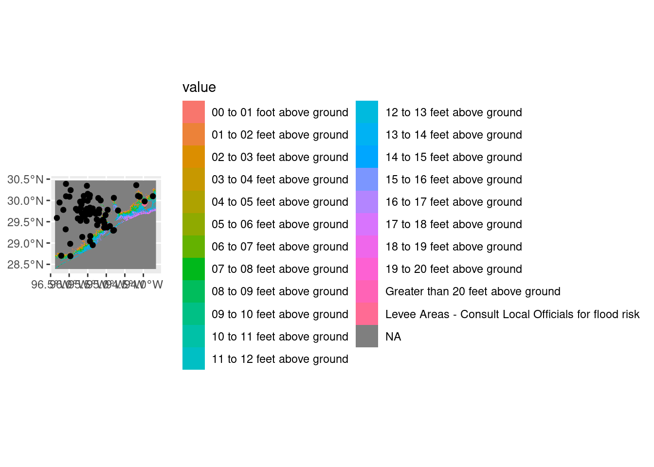
#   Extract values at church locations

foo <- cropped %>%
  terra::extract(vect(pts), method="bilinear", ID=TRUE) %>%
    group_by(ID) %>%
    summarize(value=mean(data_range, na.rm=TRUE)) %>%
  filter(!is.nan(value)) %>%
  filter(value<99) %>%
  inner_join(., Parishes, by="ID") %>%
  st_as_sf()

box <- sf::st_transform(foo, crs=inputcrs) %>%
  st_as_sf() %>% st_bbox() %>% expand_box(., 0.5)

Base_basemapR <- basemapR::base_map(box, basemap="mapnik", increase_zoom=3)


st_as_sf(foo) %>%
  ggplot() +
  Base_basemapR +
  geom_sf(color="black") +
  # geom_sf_label(aes(label=paste(stringr::str_remove(Name, "Episcopal Church"), signif(value,2)))) +
  ggsflabel::geom_sf_label_repel(aes(label=paste(stringr::str_remove(Name, "Episcopal Church"), signif(value,2), "ft"))) +
  labs(title="SLOSH model from NOAA, Cat 3 Hurricane Storm Surge in feet",
       x="Longitude",
       y="Latitude") +
  coord_sf(xlim=c(box$xmin, box$xmax),c(box$ymin, box$ymax))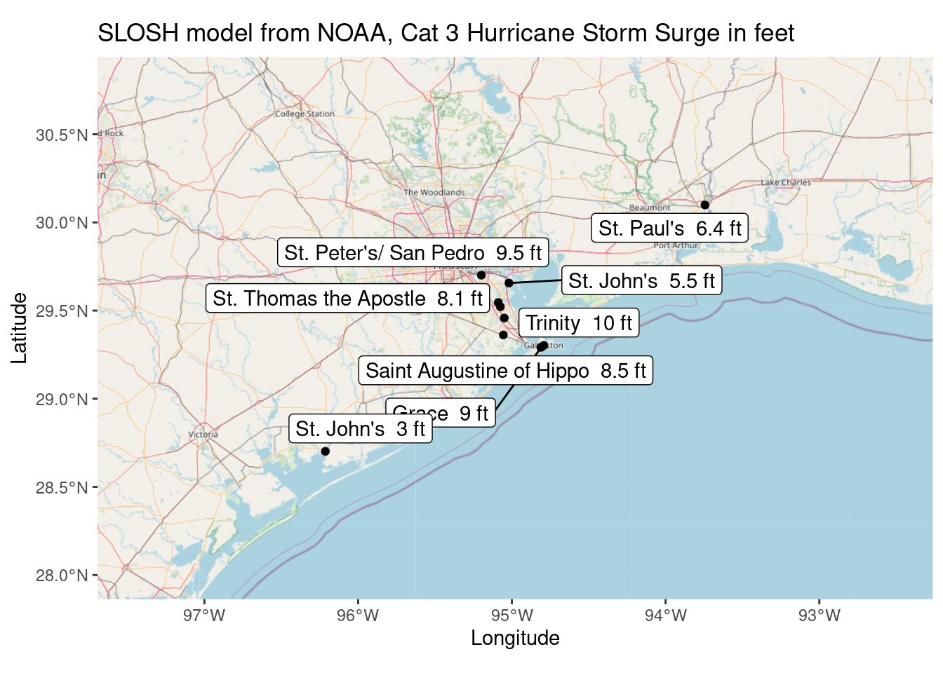
# ggsave("/home/ajackson/Desktop/Cat_1_slosh_model.jpg")Make contours (polygons) from the geotiff grid
Just to see if that would make a suitable display.
#   Make a lower resolution grid to save resources

Lowres <- cropped %>%
  aggregate(fact=10, fun="median", na.rm=TRUE) %>%
  filter(data_range<99)
|---------|---------|---------|---------|
=========================================
ggplot() +
  geom_spatraster(data=Lowres) +
  geom_sf(data=sf::st_crop(sf::st_transform(Parishes, crs=inputcrs), bbox),
          color="black")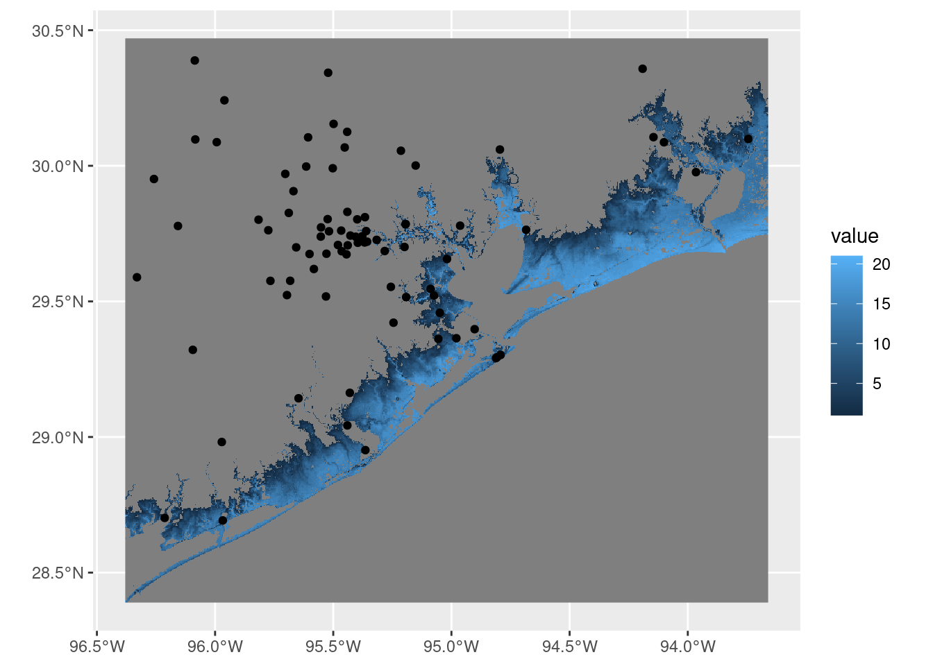
Tinybox <- bbox
Tinybox["xmin"] <- -94.868534
Tinybox["xmax"] <- -94.749265
Tinybox["ymin"] <- 29.239547
Tinybox["ymax"] <- 29.346297

ggplot() +
  basemapR::base_map(Tinybox, basemap="mapnik", increase_zoom=3)+
  geom_spatraster(data=terra::crop(Lowres, Tinybox), alpha=0.5)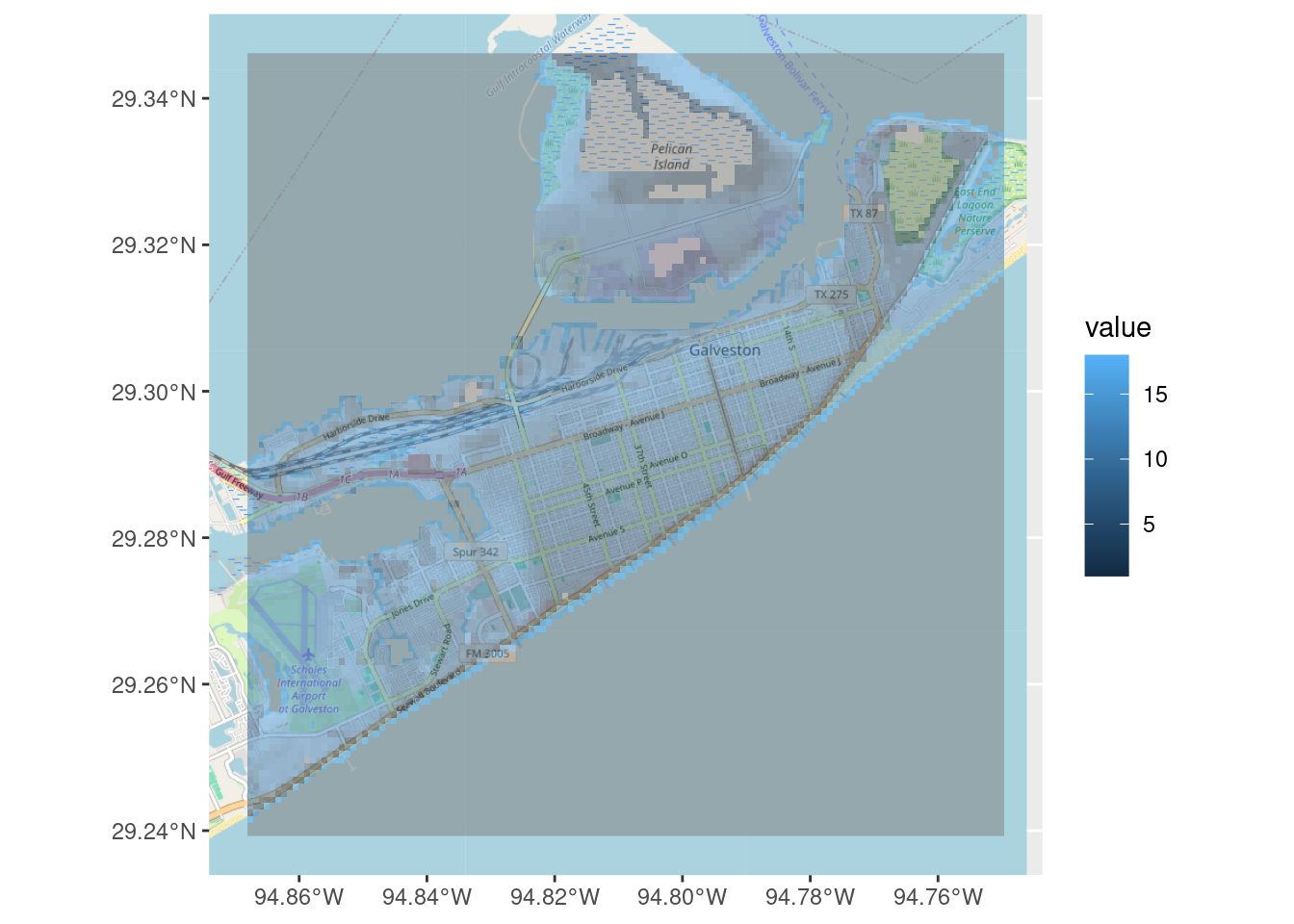
# foo_sm <- terra::focal(foo_terra, w=3, fun=mean)

LowresSm <- Lowres %>%
  terra::crop(Tinybox) %>%
  terra::focal(w=5, fun=mean, na.rm=TRUE)

Contours <- LowresSm %>%
  mapiso::mapiso() %>%
  smoothr::smooth(method="ksmooth", smoothness=2)
  # smoothr::smooth(mapiso::mapiso(terra::crop(Lowres, Tinybox)),
  #                           method="ksmooth", smoothness=2)

ggplot() +
  basemapR::base_map(Tinybox, basemap="mapnik", increase_zoom=3)+
  geom_sf(data=Contours, color="black") +
  geom_spatraster(data=terra::crop(LowresSm, Tinybox), alpha=0.2)+
  scale_fill_gradientn(colors=rainbow(5), limits=c(0,10), na.value="transparent") +
  geom_sf(data=sf::st_crop(sf::st_transform(Parishes, crs=inputcrs), Tinybox),
          color="black")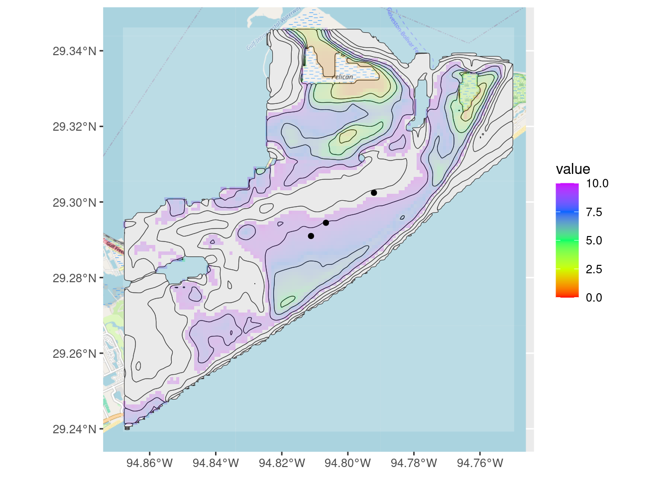
Levee polygons
Extract levees from Cat 1 file and turn into polygons
x <- terra::rast(paste0(path, "US_SLOSH_MOM_Inundation_v3/us_Category1_MOM_Inundation_HIGH.tif"))

#   Clip to AOI

cropped <- terra::crop(x, bbox)
|---------|---------|---------|---------|
=========================================
Levees <- cropped %>%
  aggregate(fact=10, fun="median", na.rm=TRUE) %>%
  filter(data_range>98) %>%
  as.polygons() %>%
  st_as_sf() %>%
  st_make_valid() %>%
  st_cast("POLYGON") %>%
  mutate(Levee_ID=row_number()) %>%
  mutate(Levee_name=case_when(
    Levee_ID==1 ~ "Port Arthur",
    Levee_ID==2 ~ "Texas City",
    Levee_ID==3 ~ "Freeport",
    Levee_ID==4 ~ "Matagorda"
  )) %>%
  filter(!is.na(Levee_name)) %>%
  select(Levee_ID, Levee_name, geometry)
|---------|---------|---------|---------|
=========================================
tmap::tmap_options(basemaps="OpenStreetMap")

tmap::tmap_mode("view") # set mode to interactive plots


tmap::tm_shape(Levees) +
  tmap::tm_fill(title = "Levees", alpha=0.5, style="cat")+
  tmap::tm_text("Levee_name")+
  tmap::tm_borders()
# saveRDS(Levees, paste0(path, "StormSurge_Levee_Polygons.rds"))Which churches are behind levees?
Make a plot of protected churches
Protected <- st_join(sf::st_transform(Parishes, crs=inputcrs), Levees, join=st_within) %>%
filter(!is.na(Levee_ID))
# Protected <- st_join(Levees, sf::st_transform(Parishes, crs=inputcrs), join=st_contains) %>%
# filter(!is.na(Levee_ID))
tmap::tmap_options(basemaps="OpenStreetMap")
tmap::tmap_mode("view") # set mode to interactive plots
tmap::tm_shape(Levees) +
tmap::tm_fill(title = "Levees", alpha=0.5, style="cat")+
tmap::tm_text("Levee_name")+
tmap::tm_borders() +
tmap::tm_shape(Protected) +
tmap::tm_dots() +
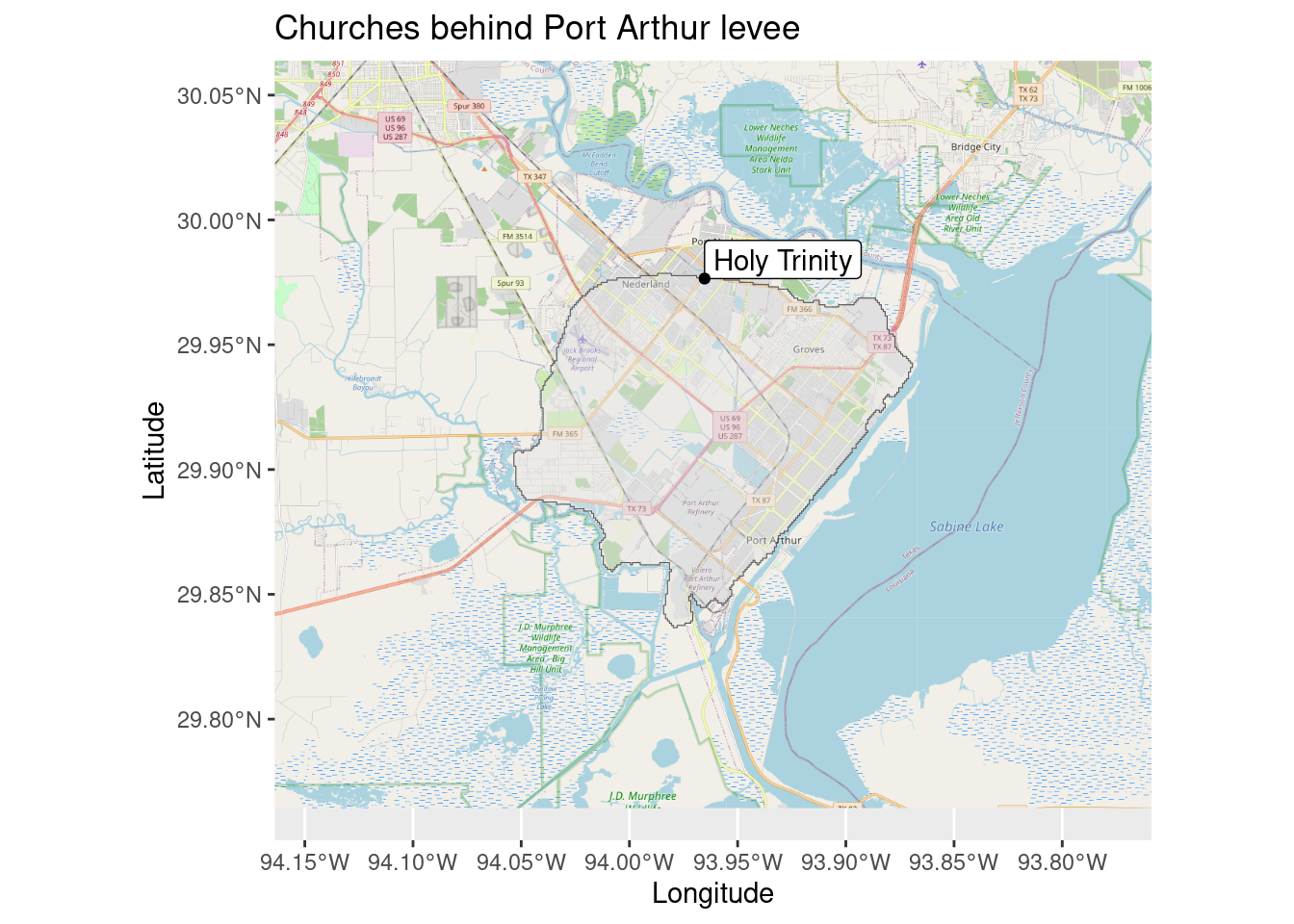
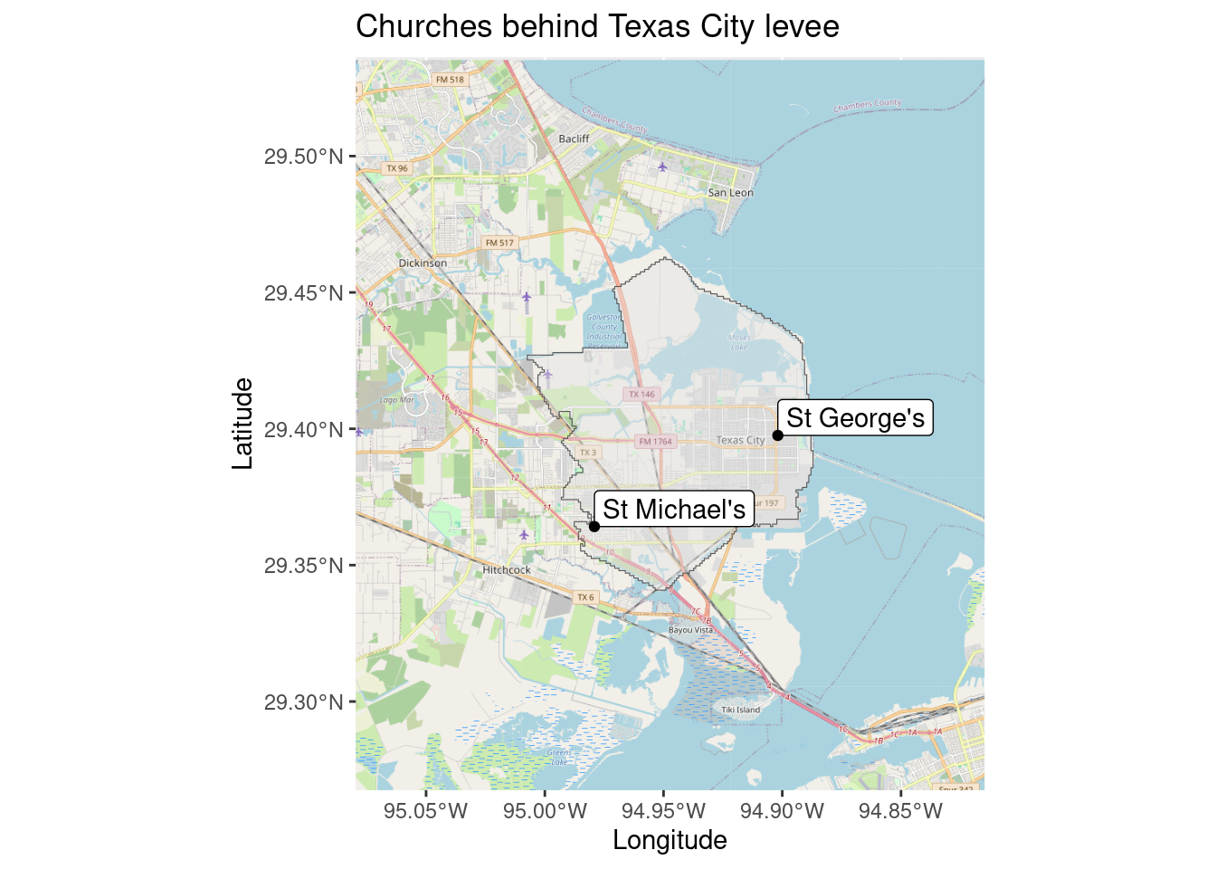
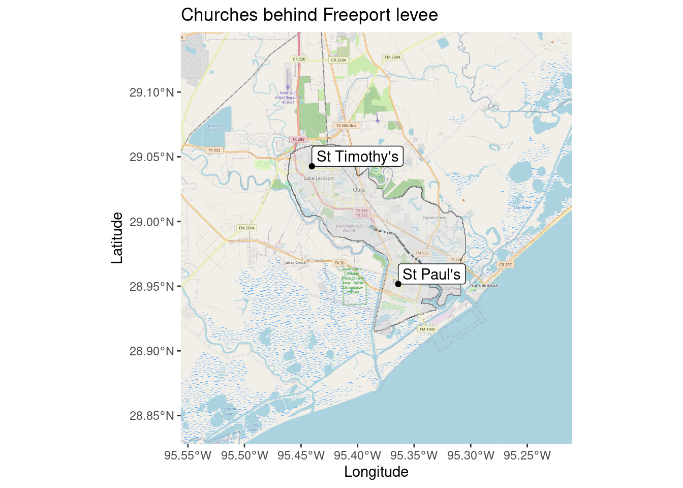
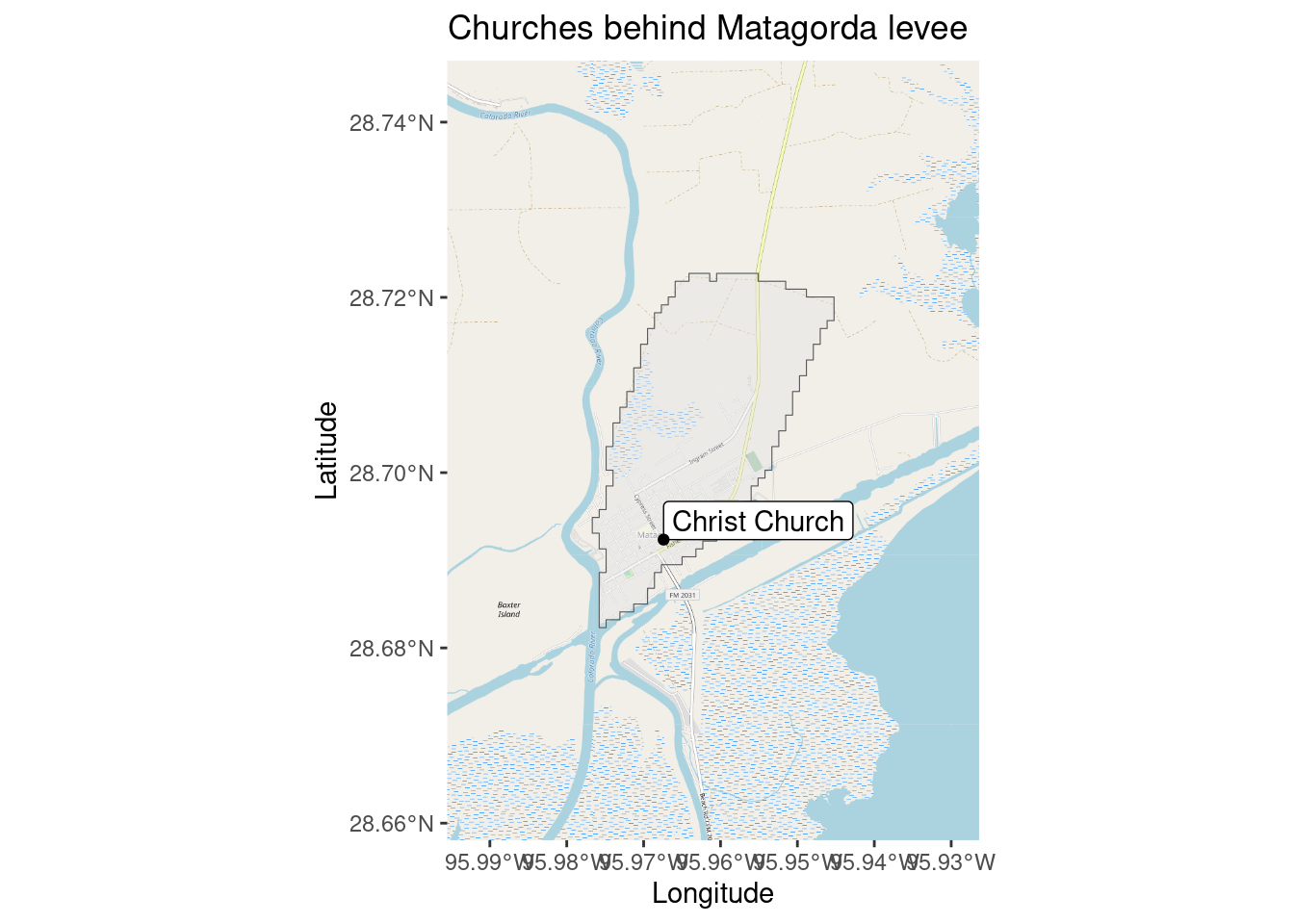
tmap::tm_text("Label", just = "left", xmod = 0.1)Make a separate plot for each levee
#   Make small maps around each of the levees showing those churches

for (Levee in c("Port Arthur", "Texas City", "Freeport", "Matagorda")){
  temp <- Protected %>%
    filter(Levee_name==Levee)

  box <- Levees %>%
    filter(Levee_name==Levee) %>%
    st_bbox() %>% expand_box(., 0.5)

  Base_basemapR <- suppressMessages(basemapR::base_map(box, basemap="mapnik", increase_zoom=3))

  print(Protected %>%
    filter(Levee_name==Levee) %>%
    ggplot() +
    Base_basemapR +
    geom_sf(data=Levees, alpha=0.4) +
    geom_sf_label(aes(label=Label),
                      hjust=0,
                      vjust=0) +
    geom_sf(color="black") +
    labs(title=paste("Churches behind", Levee, "levee"),
         x="Longitude",
         y="Latitude") +
    coord_sf(xlim=c(box$xmin, box$xmax),c(box$ymin, box$ymax))
  )
}