Read and Analyze subsidence data

Mapping

Texas

Harris county

Map the subsidence rate near Houston, Texas

Author

Alan Jackson

Published

December 16, 2023

Setup

Data scraped (with some difficulty) from https://www.arcgis.com/home/webmap/viewer.html?webmap=1e3c97ed53e2476bb842ceccd6a90514&extent=-96.3605,29.2149,-94.1042,30.3246

Found from the website for the Harris-Galveston Subsidence District.

Scraping process

Install clipit to increase clipboard buffer size
Open table
Open information screen
Find table in info screen
Select all the data with ctl-C
Dump into file with xsel -b > foo8
Shorten extremely long line with cat foo8 | sed 's/<tr>/\r<tr>/g' > foo9.html
Read into editor and add <html> <body> <table> after eliminating un-needed stuff.

library(tidyverse)

googlecrs <- "EPSG:4326"
localUTM <- "EPSG:32615"

path <- "/home/ajackson/Dropbox/Rprojects/TexasDioceseCreationCare/Data/"

Read and parse the data

# Import the data
df <- rvest::read_html(paste0(path, "SubsidenceDataHarris.html")) %>%
  rvest::html_table()

df <- do.call(rbind, df)

df <- df %>% 
  rename(Station=X1, Operator=X2, Latitude=X3, Longitude=X4, Start_Year=X5, End_Year=X6,
  Years_Monitoring=X7, Total_Vertical_Displacement_cm=X8, Subsidence_Rate_cmperyr=X9,
  POR_Plot=X10, RateLabel=X11, FID=X12
)

#   Some records are recorded at stations at the same location, which screws up kriging.
#   We will find those records and replace them with one record at that spot and average
#   the variable values.

df <- df %>% 
  mutate(index=paste0(as.character(Latitude), as.character(Longitude))) %>% 
  group_by(index) %>% 
    summarise( 
              Station=first(Station),
              Operator=first(Operator),
              Subsidence_Rate_cmperyr=mean(Subsidence_Rate_cmperyr),
              Total_Vertical_Displacement_cm=mean(Total_Vertical_Displacement_cm),
              Start_Year=min(Start_Year),
              End_Year=max(End_Year),
              Years_Monitoring=max(Years_Monitoring),
              NumInAvg=n(),
              Latitude=first(Latitude),
              Longitude=first(Longitude)) %>% 
  select(-index)

df_sf <- sf::st_as_sf(df, coords=c("Longitude", "Latitude"), crs=googlecrs, agr = "identity")
df_xy <- sf::st_transform(df_sf, crs=localUTM)

# saveRDS(df_xy, paste0(path, "Subsidence_xy.rds"))

bbox <- sf::st_bbox(df_sf)

#   Expand box by 20% to give a little extra room
Dx <- (bbox[["xmax"]]-bbox[["xmin"]])*0.1
Dy <- (bbox[["ymax"]]-bbox[["ymin"]])*0.1
bbox["xmin"] <- bbox["xmin"] - Dx
bbox["xmax"] <- bbox["xmax"] + Dx
bbox["ymin"] <- bbox["ymin"] - Dy
bbox["ymax"] <- bbox["ymax"] + Dy

bb <- c(bbox["xmin"], bbox["ymin"], bbox["xmax"], bbox["ymax"])

Plot the data

Base_basemapR <- basemapR::base_map(bbox, basemap="mapnik", increase_zoom=2)

#   This is the best looking one.
df_sf %>% 
  ggplot() +
  Base_basemapR +
  geom_sf()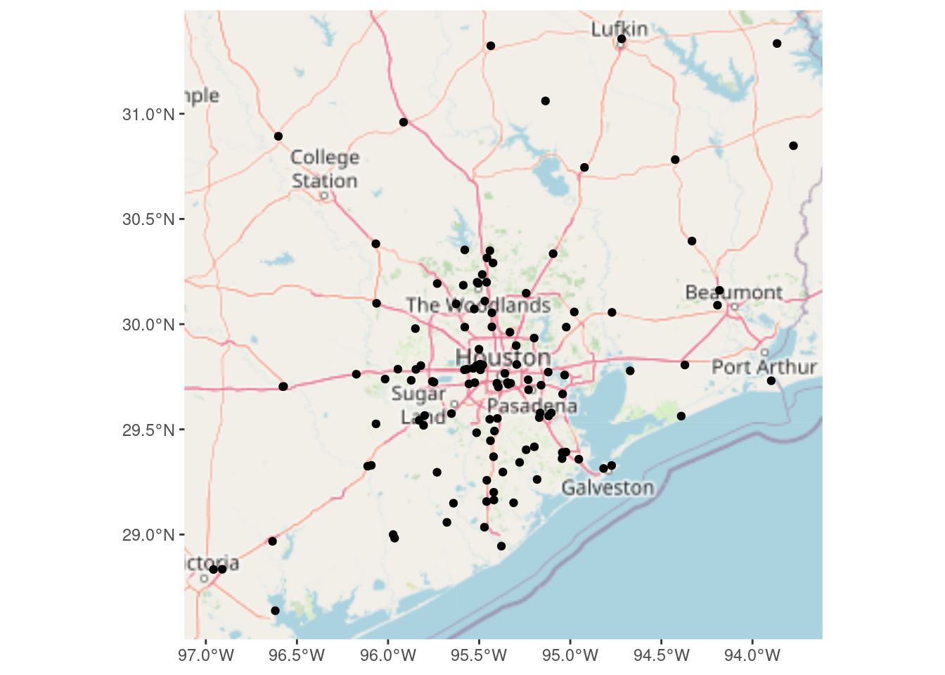

Grid and contour

Though really what I care most about is the grid, since that will yield the subsidence values at each of the church locations

#   First we create a box to build the grid inside of - in XY coordinates, not
#   lat long. 

bbox_xy = bbox %>%
  sf::st_as_sfc() %>%
  sf::st_transform(crs = localUTM) %>%
  sf::st_bbox()

#     sfc POINT file
grd_sf <- sf::st_make_grid(x=bbox_xy,
                                  what="corners",
                                  cellsize=2000,
                                  crs=localUTM
                                  )
#     Data frame
grd_df <- expand.grid(
  X = seq(from = bbox_xy["xmin"], to = bbox_xy["xmax"]+2000, by = 2000),
  Y = seq(from = bbox_xy["ymin"], to = bbox_xy["ymax"]+2000, by = 2000) # 1000 m resolution
)

Inverse distance weighting

#     Create interpolator and interpolate to grid

fit_IDW <- gstat::gstat( 
  formula = Subsidence_Rate_cmperyr ~ 1,
  data = df_xy, 
  #nmax = 10, nmin = 3, # can also limit the reach with these numbers
  set = list(idp = 2.5) # inverse distance power
)

#   Use predict to apply the model fit to the grid (using the data frame grid
#   version)

#           We set debug.level to turn off annoying output
interp_IDW <- predict(fit_IDW, grd_sf, debug.level=0)

#   Convert to a stars object so we can use the contouring in stars
interp_IDW_stars <- stars::st_rasterize(interp_IDW %>% dplyr::select(Subsidence_Rate_cmperyr=var1.pred, geometry))

#   Quick sanity check, and can use to adjust the distance power Looks pretty
#   good - most input points look close to the output grid points, with some
#   notable exceptions. The red point to the north is possibly bad data. Easier
#   to judge from areal displays.
ggplot() +
  #   geom_stars is a good way to display a grid
  stars::geom_stars(data=interp_IDW_stars) +  
  geom_sf(data=df_xy, aes(color=Subsidence_Rate_cmperyr), size=5) +
  geom_sf(data=df_xy, color="Black", size=1) +
  #     This is for the raster color fill
  scale_fill_gradientn(colors=rainbow(5), limits=c(-2,1)) +
  #     This is for the original data points
  scale_color_gradientn(colors=rainbow(5), limits=c(-2,1)) +
  labs(title="Inverse Distance Weighting, Power = 2.5")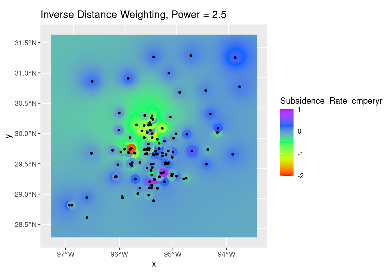

Search for best IDW power

Even optimizing, the result is kind of sucky.

#   Do a leave-one-out analysis for a variety of weighting powers
Validate <- NULL
for (power in (2:8)*0.5) {
  my_fit <- gstat::gstat(formula = Subsidence_Rate_cmperyr ~ 1, data = df_xy,  set = list(idp = power))
  foo <- sf::st_as_sf(gstat::gstat.cv(my_fit, debug.level=0, verbose=FALSE)) %>% 
    rename(Observed=observed, Predicted=var1.pred ) %>% 
    mutate(power=power) 
  
  Validate <- bind_rows(Validate, foo)
}

Validate %>% 
  ggplot(aes(x=Observed, y=Predicted)) + 
    geom_point() +
    geom_smooth(method='lm') +
    geom_abline(intercept=0, slope=1, color="red", linetype="dashed") +
    facet_wrap(vars(power)) +
    labs(title="Leave-one-out Validation",
         x="Observed (inches)",
         y="Predicted (inches)")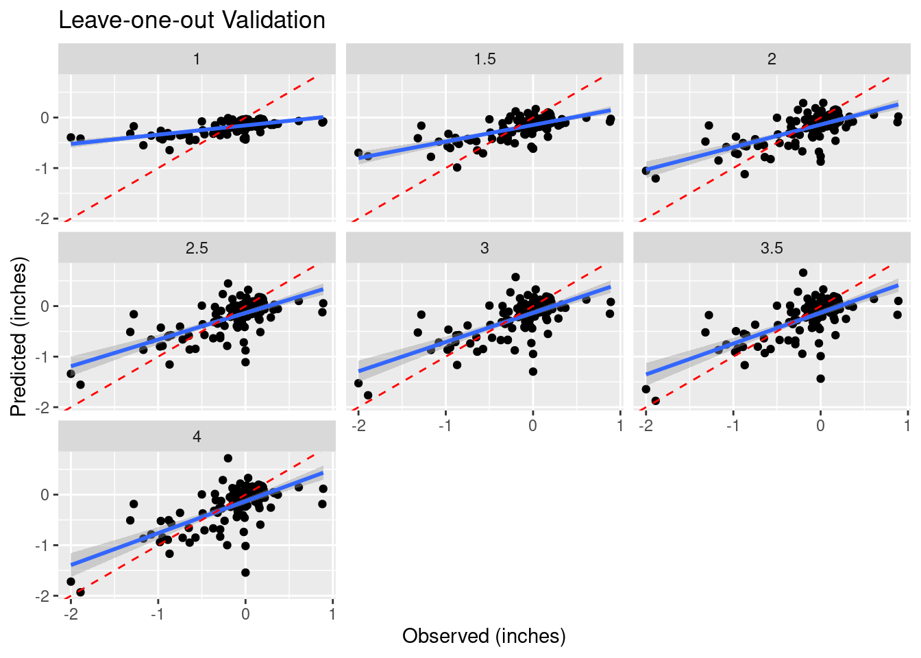

#     Root mean square error

RMS <- Validate %>% 
  group_by(power) %>% 
  summarise(RMS=sqrt(sum((Predicted-Observed)^2) / n()))

RMS %>% 
  ggplot(aes(x=power, y=RMS)) +
    geom_point() +
    geom_smooth() +
    labs(title="RMS Error vs. Inverse Distance Weighting Power")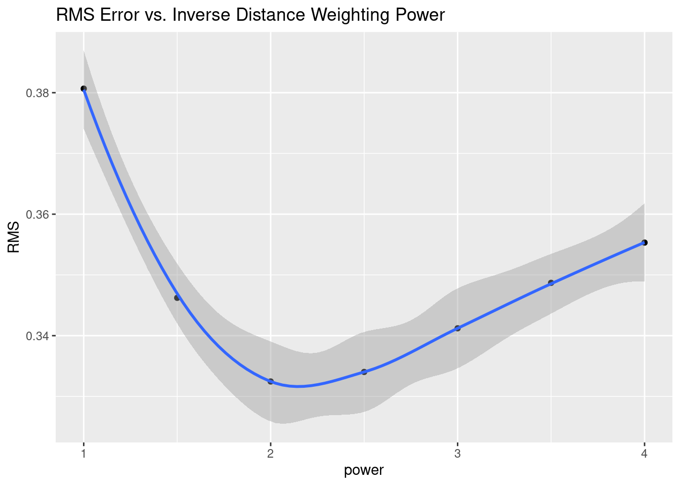

Kriging

First the drift.

I don’t like the looks of the fit - I think that there is enough data surrounding the bowl near zero that there is no drift. This is a flat plane with a bowl in the middle.

#   Let's look at 1st order fit

df_xy_df <- bind_cols(sf::st_drop_geometry(df_xy), 
                      sf::st_coordinates(df_xy)) # make a tibble

# Define the 1st order polynomial equation
f.1 <- as.formula(Subsidence_Rate_cmperyr ~ X + Y) 

# Run the regression model
lm.1 <- lm( f.1, data=df_xy_df)

#   Use predict to apply the model fit to the grid This re-attaches X-Y
#   coordinates to the predicted values so they can be made into a grid

Poly_fit.1 <- sf::st_as_sf(bind_cols(grd_df,
                                     data.frame(var1.pred=predict(lm.1, grd_df))), 
                           crs=localUTM, 
                           coords=c("X", "Y"))

#   Convert to a stars object 
Poly_fit_star.1 <- stars::st_rasterize(Poly_fit.1 %>% 
                                         dplyr::select(Subsidence_Rate_cmperyr=var1.pred, geometry))

ggplot() +
  stars::geom_stars(data=Poly_fit_star.1) +
  scale_fill_gradientn(colors=rainbow(5)) +
  geom_sf(data=df_xy, aes(color=Subsidence_Rate_cmperyr), size=5) +
  scale_color_gradientn(colors=rainbow(5), limits=c(-2,1)) +
  scale_fill_gradientn(colors=rainbow(5), limits=c(-2,1)) +
  geom_sf(data=df_xy, color="Black", size=1)+ 
  labs(title="Linear trend from subsidence data")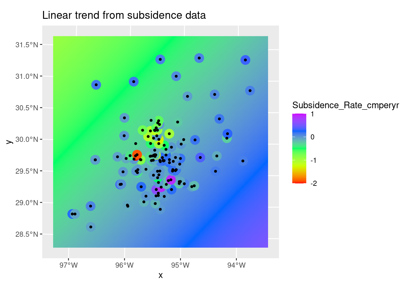

Kriging

I pick the Spherical model

#   Let's look at the variogram

var.smpl <- gstat::variogram(Subsidence_Rate_cmperyr ~ 1, 
                             data=df_xy)
# Compute the variogram model by passing the nugget, sill and range values
# to fit.variogram() via the vgm() function.
#                models are "Sph", "Exp", "Mat", and "Gau"

Plot_data <- NULL
for (model in c("Sph", "Exp", "Mat", "Gau")) {
  foo  <- gstat::fit.variogram(var.smpl, fit.ranges = TRUE, fit.sills = TRUE,
                                   debug.level = 0,
                            gstat::vgm(psill=NA, model=model, range=NA, nugget=0))
  Plot_data <- bind_rows(Plot_data, gstat::variogramLine(foo, maxdist = max(var.smpl$dist)) %>% 
                           mutate(Model=model))
}

ggplot(var.smpl, aes(x = dist, y = gamma)) +
     geom_point() +
     geom_text(aes(hjust="left", label=np), nudge_x=200) +
     geom_line(data=Plot_data, aes(x=dist, y=gamma, color=Model)) +
     labs(title="Variogram for detrended data",
          subtitle="Numbers represent number of points in the distance bin")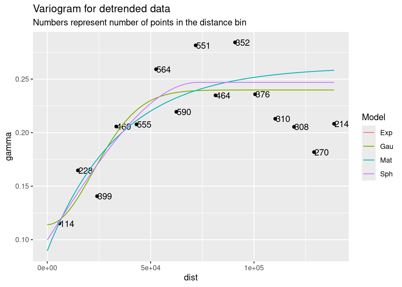

Do Kriging

#   We have our model, so now let's use it
dat.fit <- gstat::fit.variogram(var.smpl, fit.ranges = TRUE, fit.sills = TRUE,
                                   debug.level = 0,
                            gstat::vgm(psill=NA, model="Gau", range=NA, nugget=0))

# saveRDS(dat.fit, paste0(path, "gstat_variogram_Subsidence.rds"))

Krigged_grid <- gstat::krige(Subsidence_Rate_cmperyr ~ 1,
                             df_xy,
                             grd_sf,
                             debug.level=1,
                             dat.fit)

[using ordinary kriging]

Krigged_star <- stars::st_rasterize(Krigged_grid %>% dplyr::select(Subsidence_Rate_cmperyr=var1.pred, geometry))

#     Residuals
ggplot() +
  stars::geom_stars(data=Krigged_star) +
  scale_fill_gradientn(colors=rainbow(5)) +
  geom_sf(data=df_xy, color="Black", size=1) +
  labs(title="Residuals from Kriging")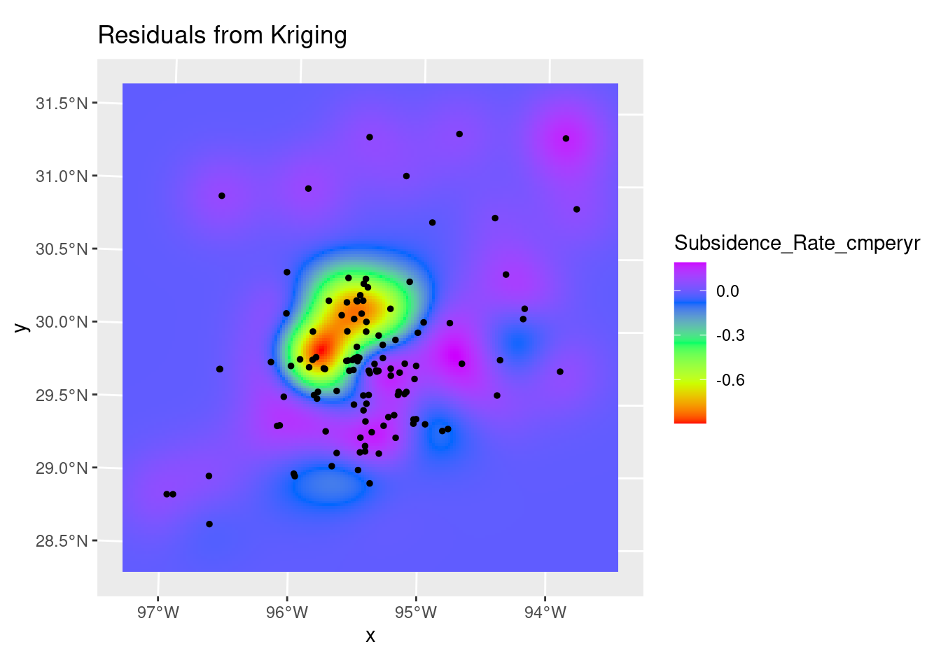

Contours

brks <- seq(from = -1, to = 0.2, by = 0.2)
#   Create contour lines
Contours_Krig <- stars::st_contour(Krigged_star, contour_lines=TRUE, breaks=brks)
#   Plot to see what it all looks like
ggplot() +
  stars::geom_stars(data=Krigged_star) +
  scale_fill_gradientn(colors=rainbow(5), limits=c(-1,0.2)) +
  geom_sf(data=df_xy, aes(color=Subsidence_Rate_cmperyr), size=5) +
  scale_color_gradientn(colors=rainbow(5), limits=c(-1,0.2)) +
  geom_sf(data=df_xy, color="Black", size=1) +
  geom_sf(data=Contours_Krig, color="black")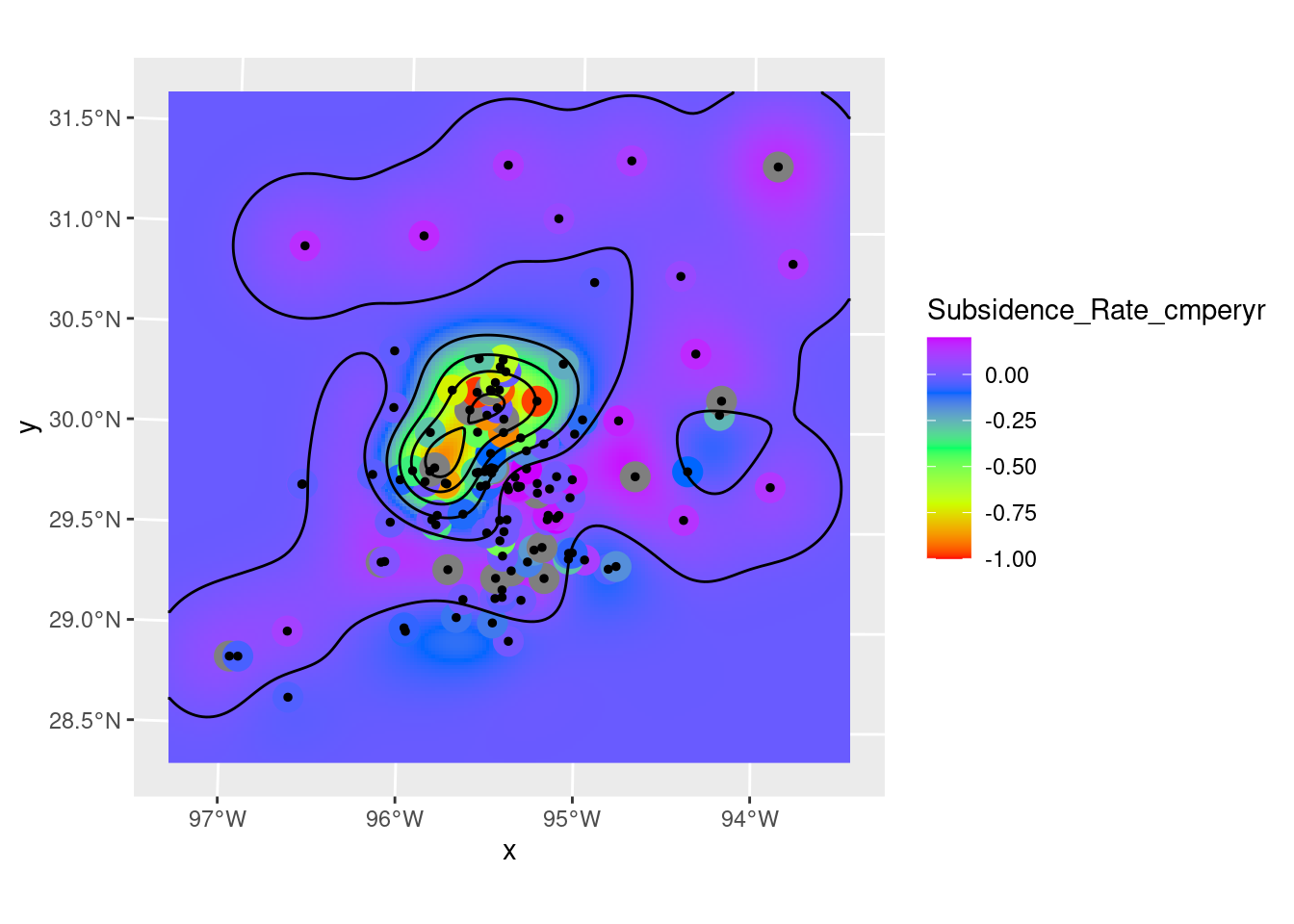

Final publication quality map

#   Now lets transform the contours to lat-long space and plot on the basemap

Contours_LL <- sf::st_transform(Contours_Krig, crs=googlecrs) 
Krig_star_LL <- sf::st_transform(Krigged_star, crs=googlecrs)

# saveRDS(Contours_LL, paste0(path, "Contours_LL_Subsidence.rds"))
# saveRDS(Krig_star_LL, paste0(path, "Star_Grid_LL_Subsidence.rds"))

ggplot() +
  #   this is the best looking basemap
  Base_basemapR +
  #   Gridded data
  stars::geom_stars(data=Krig_star_LL, alpha=0.4) +  
  #   Add points
  geom_sf(data=df_sf) +
  #   Create filled density "contours" 
  geom_sf(data=Contours_LL, color="black") +
  scale_fill_viridis_c(direction=-1, alpha=0.4, name="Subsidence\nRate (cm/yr)") +
  #   Add a scale bar
  ggspatial::annotation_scale(data=df_sf, aes(unit_category="imperial", style="ticks"),
    location="br", width_hint=0.2, bar_cols=1) +
  #   Add CI annotation at specified window coordinates
  annotate("text", label="C.I. = 0.2 cm per year subsidence
           Data sourced from the Harris-Galveston Subsidence District 
           2022 Annual Groundwater Report
           Map a product of Alan Jackson", 
           x=-Inf, 
           y=-Inf,
           hjust="inward", vjust="inward", size = 2) +
  coord_sf(crs=googlecrs) + # required 
  #   Add title
  labs(title="Subsidence Rate",
       subtitle="Points represent the measurement locations",
       x="Longitude", y="Latitude")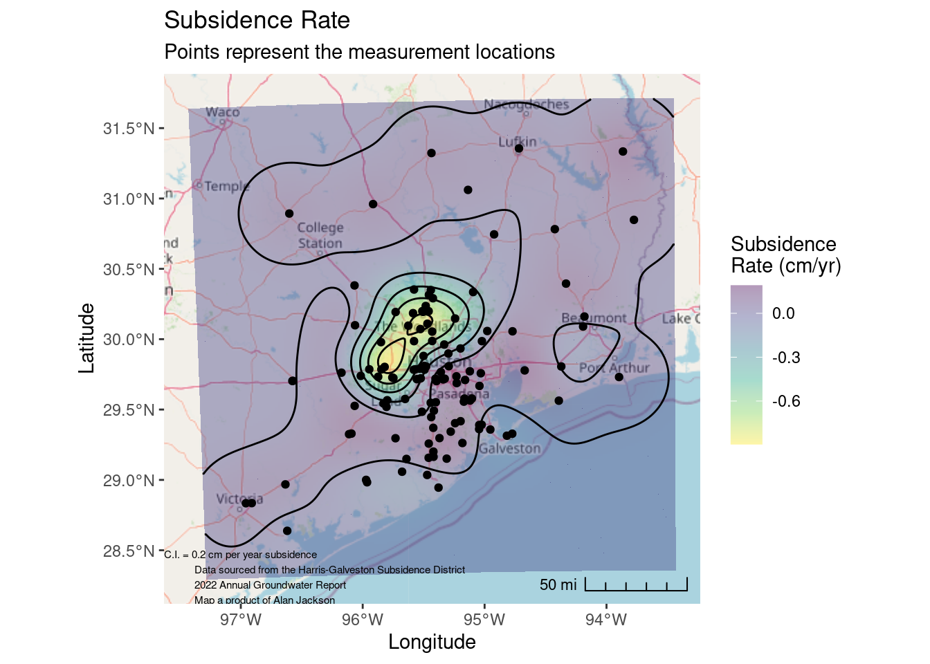

# ggsave(paste0(path, "Subsidence_map.png"),dpi=400)