How close are reported Texas measles cases fitting an exponential?
Author
Alan Jackson
Published
April 20, 2025
Is the measles epidemic in Texas showing exponential growth?
I got curious about the growth rate of infections, and if it was exponential what the doubling time would be. So I downloaded some data and did a quick analysis.
Data downloaded from this page: https://www.dshs.texas.gov/news-alerts/measles-outbreak-2025
Code
library(tidyverse)path <-"/home/ajackson/Dropbox/"df <-read_csv(paste0(path, "Figure 15 Epi Curve of Cases by Rash Onset Date (2_data.csv"))df <- df %>%mutate(Date=mdy(`Day of Epi Curve Date`)) %>%arrange(Date) %>%mutate(Cumulative=cumsum(Confirmed)) %>%mutate(Day=as.numeric(Date-first(Date))) %>%mutate(Cumulative2=cumsum(Confirmed*2))
Fit the data
Do a linear, an exponential, and a logistic fit to the data
Code
# These are "gapless" sequences, since there are a few gaps in the original # datadayseq <-0:last(df$Day)Dateseq <-first(df$Date) + dayseq########## Linearmodel1 =lm(Cumulative ~ Day, data = df)m <- model1[["coefficients"]][["Day"]]b <- model1[["coefficients"]][["(Intercept)"]]Rsqr1 <-summary(model1)$adj.r.squaredstd_dev1 <-sigma(model1)# Calculate the fitted valuesCases1 <- m*dayseq+b# Create a dataframe of the fitcase_fit1 <<-tibble(Model="Linear", Days=dayseq, Date=Dateseq, Cases=Cases1)# upper_conf=Cases1+std_dev, lower_conf=Cases1-std_dev) ########## Exponentialmodel2 <-lm(log10(Cumulative)~Day, data=df)m <- model2[["coefficients"]][["Day"]]b <- model2[["coefficients"]][["(Intercept)"]]Rsqr2 <-summary(model2)$adj.r.squaredstd_dev2 <-sigma(model2)# Calculate the fitted valuesCases2 <-10**(m*dayseq+b)# Create a dataframe of the fitcase_fit2 <<-tibble( Model="Exponential", Days=dayseq, Date=Dateseq, Cases=Cases2)# upper_conf=Cases2+std_dev, lower_conf=Cases2-std_dev) ########## Logistic# Initialize for non-linear fitAsym <-max(df$Cumulative)*5xmid <-max(df$Days)*2scal <-1/0.24my_formula <-as.formula("Cumulative ~ SSlogis(Day, Asym, xmid, scal)")logistic_model <-nls(my_formula, data=df)coeffs <-coef(logistic_model)Cases3 <-predict(logistic_model, data.frame(Day=dayseq))case_fit3 <-tibble(Model="Logistic", Date=Dateseq, Days=dayseq, Cases=Cases3)# Build a dataframe of fitsAll_fits <-rbind(case_fit1, case_fit2, case_fit3) # Calculate deviations between fits and dataDeviation <- All_fits %>%right_join(., df, by="Date") %>%group_by(Model) %>%summarise(SumDev=signif(sum(abs(Cases-Cumulative)),3))
Make some plots
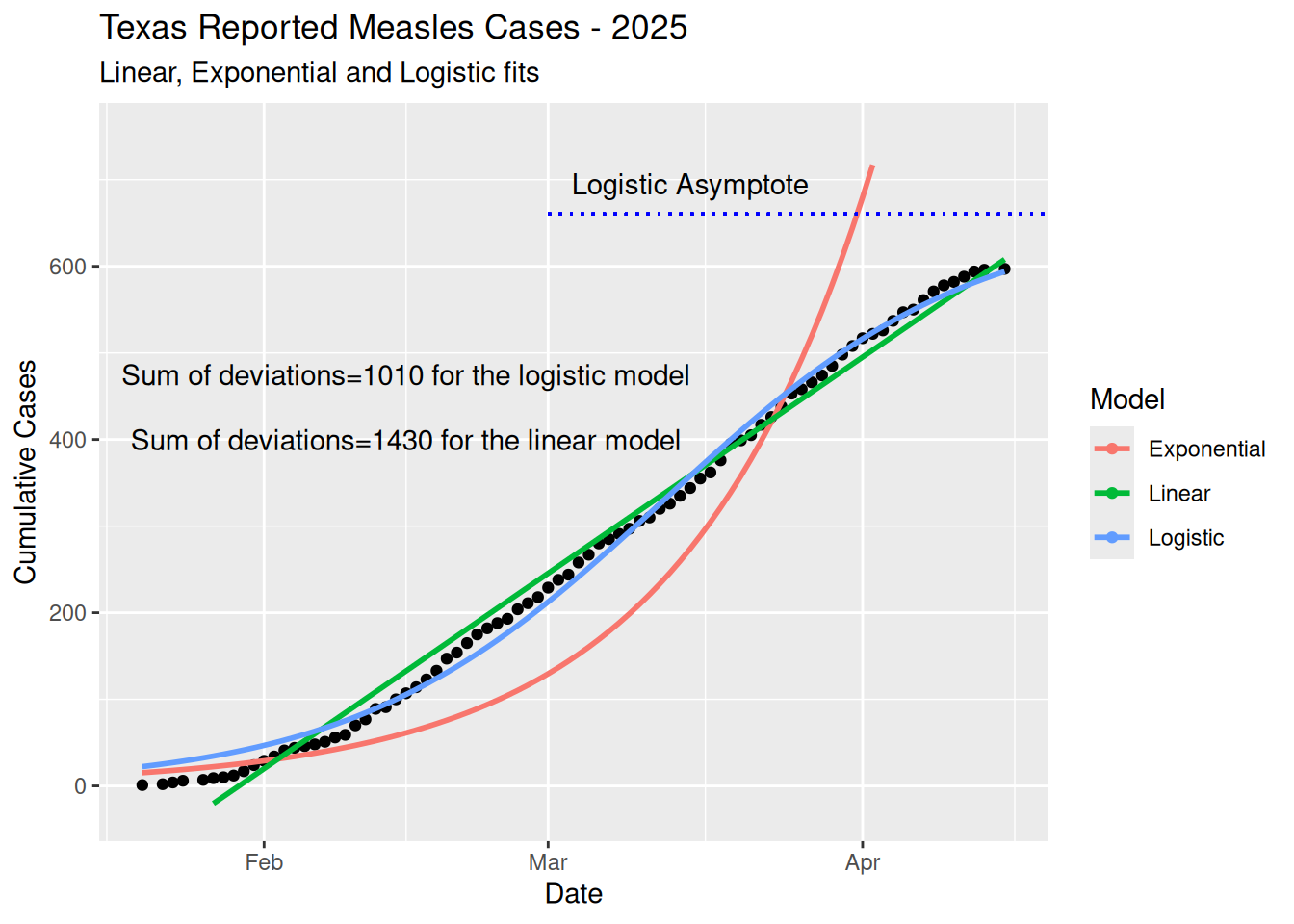
It appears that an exponential is a terrible fit for the data. On the other hand, a simple linear fit is pretty awesome. But the logistic seems perhaps even better. If so, then it might indicate that the epidemic is tailing off and may end soon. One can only hope. The logistic does yield a somewhat smaller sum of deviations from the input data, for what it is worth.
Code
Asymp <- coeffs[[1]]All_fits %>%ggplot(aes(x=Date, y=Cases, color=Model)) +scale_y_continuous(limits =c(-25, 750)) +geom_point(data=df, aes(x=Date, y=Cumulative, group=NULL, color=NULL)) +geom_line(linewidth=1) +annotate("text", ymd("2025-Mar-15"), y=Asymp+35, label="Logistic Asymptote") +geom_segment(x =ymd("2025-Mar-1"), y = Asymp, linetype="dotted",xend =ymd("2025-4-25"), yend = Asymp, color ="blue") +annotate("text", ymd("2025-2-15"), y=400,label=paste0("Sum of deviations=", Deviation[2,2], " for the linear model"))+annotate("text", ymd("2025-2-15"), y=475,label=paste0("Sum of deviations=", Deviation[3,2], " for the logistic model"))+# geom_smooth(data=df, aes(x=Date, y=Cumulative), method = "lm") +# geom_line(data=case_fit2, aes(x=Date, y=Cases), color="red") +labs(title="Texas Reported Measles Cases - 2025",subtitle="Linear, Exponential and Logistic fits",y="Cumulative Cases")