Harris County School Districts

Create polygon files of school districts in Harris county and intersect with zipcodes.

Prepare data for analyzing zipcode-based data by school district

During COVID, at one point, Harris county began to supply infection rates daily by zip code. At about the same time, different school districts in the area developed wildly differing policies on returning to in-person instruction, masking, etc. In order to study those differences I needed to be able to take the COVID data by zip code and interpolate it into the various districts. That is the purpose of this exercise.

First let’s get the school districts read in and cleaned up

Data was downloaded in 2019 from the Texas Education Agency website at https://schoolsdata2-tea-texas.opendata.arcgis.com/datasets/36b0225013a04341bb49b98155186863/explore as a shapefile.

The proj file indicates that the data is in EPSG 4326 - same as Google Maps, so Yay!

#   Read in the shapefiles
SchoolPolys <- read_sf(paste0(path,"SchoolDistricts/Current_Districts.shp"))

summary(SchoolPolys)

      FID         SDLEA10              NAME              NAME2          
 Min.   :   1   Length:1021        Length:1021        Length:1021       
 1st Qu.: 256   Class :character   Class :character   Class :character  
 Median : 511   Mode  :character   Mode  :character   Mode  :character  
 Mean   : 511                                                           
 3rd Qu.: 766                                                           
 Max.   :1021                                                           
   DISTRICT_N       DISTRICT          DISTRICT_C         NCES_DISTR       
 Min.   :  1902   Length:1021        Length:1021        Length:1021       
 1st Qu.: 64903   Class :character   Class :character   Class :character  
 Median :117904   Mode  :character   Mode  :character   Mode  :character  
 Mean   :125557                                                           
 3rd Qu.:184902                                                           
 Max.   :254902                                                           
     COLOR         SHAPE_Leng       SHAPE_Area                 geometry   
 Min.   :1.000   Min.   :0.0456   Min.   :1.272e+06   MULTIPOLYGON :1021  
 1st Qu.:2.000   1st Qu.:0.8799   1st Qu.:2.100e+08   epsg:4326    :   0  
 Median :4.000   Median :1.2803   Median :3.936e+08   +proj=long...:   0  
 Mean   :3.984   Mean   :1.4230   Mean   :6.795e+08                       
 3rd Qu.:6.000   3rd Qu.:1.8629   3rd Qu.:7.842e+08                       
 Max.   :7.000   Max.   :5.1094   Max.   :1.254e+10                       

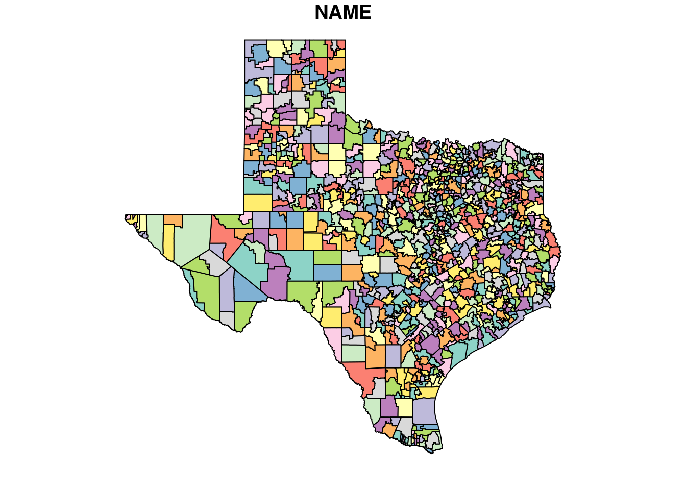
#   CRS is good, we have polys, I think I'm happy. Let's plot them

plot(SchoolPolys[,"NAME"])

#   So this is all districts in Texas. How do I carve out Harris county?
#   I guess by intersecting with Harris county

Harris <- readRDS(paste0(path,"HarrisCounty_16.rds"))

sf::st_crs(Harris) <- googlecrs

old-style crs object detected; please recreate object with a recent sf::st_crs()

Warning: st_crs<- : replacing crs does not reproject data; use st_transform for
that

summary(Harris)

    County             Tract              BlkGrp              MedAge     
 Length:2539        Length:2539        Length:2539        Min.   :12.20  
 Class :character   Class :character   Class :character   1st Qu.:30.70  
 Mode  :character   Mode  :character   Mode  :character   Median :36.05  
                                                          Mean   :37.22  
                                                          3rd Qu.:42.70  
                                                          Max.   :83.00  
                                                          NA's   :3      
  MedAgeSigma       MedAgeMale     MedAgeFemale        Pop         
 Min.   : 0.200   Min.   : 7.70   Min.   :12.80   Min.   :    0.0  
 1st Qu.: 4.100   1st Qu.:29.50   1st Qu.:30.90   1st Qu.:  993.5  
 Median : 6.800   Median :34.90   Median :37.20   Median : 1407.0  
 Mean   : 7.924   Mean   :36.06   Mean   :38.23   Mean   : 1683.0  
 3rd Qu.:10.400   3rd Qu.:41.92   3rd Qu.:44.60   3rd Qu.: 2049.0  
 Max.   :48.200   Max.   :85.60   Max.   :82.30   Max.   :17391.0  
 NA's   :3        NA's   :3       NA's   :5                        
    PopSigma          White             Black           Amerind       
 Min.   :  13.0   Min.   :    0.0   Min.   :   0.0   Min.   :  0.000  
 1st Qu.: 261.5   1st Qu.:  730.5   1st Qu.:   5.5   1st Qu.:  0.000  
 Median : 357.0   Median : 1069.0   Median :  66.0   Median :  0.000  
 Mean   : 390.9   Mean   : 1259.5   Mean   : 206.1   Mean   :  8.259  
 3rd Qu.: 479.0   3rd Qu.: 1535.5   3rd Qu.: 255.5   3rd Qu.:  4.000  
 Max.   :3022.0   Max.   :12241.0   Max.   :3025.0   Max.   :514.000  
                                                                      
     Asian            Hispanic        MedIncome      MedIncomeSigma  
 Min.   :   0.00   Min.   :   0.0   Min.   :  5491   Min.   :  1246  
 1st Qu.:   0.00   1st Qu.: 173.0   1st Qu.: 36698   1st Qu.:  9523  
 Median :   7.00   Median : 410.0   Median : 51704   Median : 14869  
 Mean   :  70.69   Mean   : 613.0   Mean   : 60642   Mean   : 18716  
 3rd Qu.:  66.00   3rd Qu.: 839.5   3rd Qu.: 72434   3rd Qu.: 23232  
 Max.   :2249.00   Max.   :8892.0   Max.   :250001   Max.   :156982  
                                    NA's   :71       NA's   :81      
           Shape     
 MULTIPOLYGON :2539  
 epsg:4326    :   0  
 +proj=long...:   0  
                     
                     
                     
                     

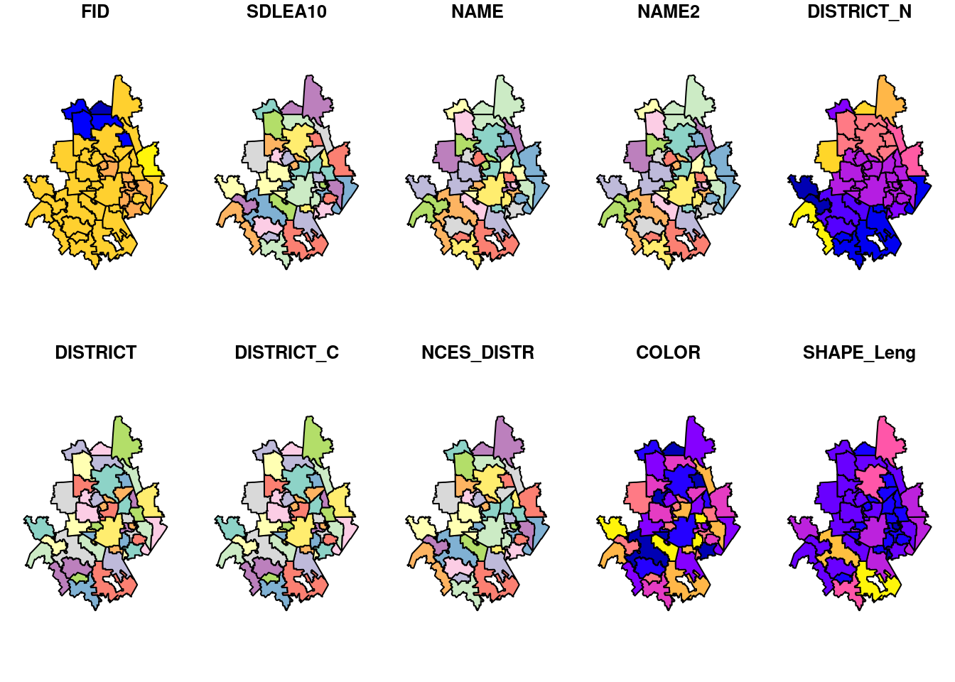
# convert to proper EPSG

Harris <- st_transform(Harris, googlecrs)

foo <- sf::st_make_valid(SchoolPolys)[Harris,]

plot(foo)

Warning: plotting the first 10 out of 11 attributes; use max.plot = 11 to plot
all

leaflet::leaflet(foo) %>% 
        leaflet::setView(lng = -95.3103, lat = 29.7752, zoom = 8 ) %>%   
        leaflet::addTiles() %>%
        leaflet::addPolygons(data = foo, 
                    weight = 1,
                    smoothFactor = 0.2, 
                    fillOpacity = 0.5,
                    fillColor =  foo$COLOR) %>% 
        leaflet::addPolygons(data = Harris, 
                    weight = 1,
                    smoothFactor = 0.2, 
                    fillOpacity = 0.2,
                    fillColor =  "red")  

#   Let's see if we can just extract the districts using my list

Districts <- c("Aldine", "Alief", "Channelview", "Crosby",
"Cypress-Fairbanks", "Deer Park", "Galena Park", "Goose Creek Cons",
"Houston", "Humble", "Klein", "La Porte", "Pasadena", "Sheldon",
"Spring", "Spring Branch", "Clear Creek", "Katy")

foo <- SchoolPolys[SchoolPolys$NAME2 %in% Districts,]

#   Better. Let's save the polygon file, with NAME2

foo <- foo %>% 
  select(-FID, -SDLEA10, -NAME, -DISTRICT_N, -DISTRICT, -DISTRICT_C, 
         -NCES_DISTR, -COLOR) %>% 
  rename(District=NAME2)

#   Save districts that intersect Harris county 

saveRDS(foo, paste0(path, "SchoolDistricts/HarrisCtySchools.rds"))

Now let’s build a weight table of zipcodes in each district

Want to be able to adjust each district by what fraction of it lies in Harris county zipcodes.

Zip_poly <- readRDS(paste0(path, "ZipCodes_sf.rds"))
sf::st_crs(Zip_poly) <- googlecrs

old-style crs object detected; please recreate object with a recent sf::st_crs()

Zip_poly <- sf::st_make_valid(Zip_poly)

intersect <- st_intersection(foo, Zip_poly)

Warning: attribute variables are assumed to be spatially constant throughout
all geometries

answer <- intersect %>% 
  mutate(area=st_area(.) %>% as.numeric()) %>% 
  as_tibble() %>% 
  group_by(Zip_Code, District) %>% 
  summarize(area = sum(area))

`summarise()` has grouped output by 'Zip_Code'. You can override using the
`.groups` argument.

answer <- answer %>% 
  group_by(Zip_Code) %>% 
    mutate(total_area=sum(area)) %>% 
    mutate(fraction_of_zip=area/total_area) %>% 
  ungroup() 

saveRDS(answer, paste0(path,"SchoolDistricts/Fraction_Zip_Per_School_District.rds"))

Now let’s read in all the census data and create files by

Zipcode and by District from that

Don’t forget the blueness too!

Already have data by zip. Hmmm….. not quite the best thing, but instead of tracking down the data by block, let’s just go from zipcode to district.

#   Census data for 2016

Zip_census16 <- readRDS(paste0(path, "TexasZipcode_16.rds"))
Zip_census16 <- Zip_census16 %>% 
  mutate(ZCTA=as.character(ZCTA))

#   Median family income and number of families
Income <- readRDS("/home/ajackson/Dropbox/Rprojects/Datasets/IncomeByZip.rds")

#   Many vs 2 generational households
House <- readRDS("/home/ajackson/Dropbox/Rprojects/Datasets/HouseholdByZip.rds")

#   Blueness

Blueness <- readRDS(paste0(path,"HarrisBlueness.rds")) 

# First create files by zip - polygon and data

DF_values <- Zip_census16 %>% 
  select(-MalePop) %>% 
  mutate(MedianAge=as.numeric(MedianAge))

Warning: There was 1 warning in `mutate()`.
ℹ In argument: `MedianAge = as.numeric(MedianAge)`.
Caused by warning:
! NAs introduced by coercion

DF_values <- left_join(DF_values, Income, by="ZCTA")

DF_values <- left_join(DF_values, House, by="ZCTA")

# Drop NA will restrict to Harris county

DF_values <- left_join(DF_values, Blueness, by="ZCTA") %>% 
  drop_na()

DF_values <- DF_values %>% 
  mutate(WhitePct=White/Pop*100, 
         BlackPct=Black/Pop*100, 
         HispanicPct=Hispanic/Pop*100,
         MultigenPct=Households_threegen/Total_Households*100)

left_join.sf =
  function(x,y,by=NULL,copy=FALSE,suffix=c(".x",".y"),...){
  ret = NextMethod("left_join")
  sf::st_as_sf(ret)
}

Zip_poly <- sf::st_as_sf(Zip_poly)

DF_values <- left_join(DF_values, Zip_poly, by=c("ZCTA"="Zip_Code")) %>% 
  mutate(Density=5280*5280*Pop/Shape_Area) %>%  # per sq mile
  select(-Shape) %>% 
  as_tibble()

DF_polys <- left_join(DF_values, Zip_poly, by=c("ZCTA"="Zip_Code"))  
DF_polys <- sf::st_as_sf(DF_polys)

#   Save files out

saveRDS(DF_values, paste0(path, "HarrisCounty_CensusByZip.rds"))
saveRDS(DF_polys, paste0(path, "HarrisCounty_CensusByZip_polys.rds"))

##########   Now do School Districts

foo2 <- left_join(answer, foo, by="District") %>% 
  left_join(., DF_values, by=c("Zip_Code"="ZCTA"))  

Mult_by <- function(a, frac){ a*frac }

by_mean <- c("MedianAge", "Med_Income", "blueness")
by_sum <- c("Pop", "Age0to4", "Age5to9", "Age10to14", "Age15to19",
            "Age20to24", "Age25to34", "Age35to44", "Age45to54", "Age55to59",
            "Age60to64", "Age65to74", "Age75to84",  "Age85andup", "White", 
            "Black", "Hispanic",  "Number_Families", "Total_Households",
            "Households_threegen", "Households_twogen", "total_vote")

Sums <- foo2 %>% 
  group_by(District) %>% 
    transmute_at(by_sum, funs(Mult_by(.,fraction_of_zip))) %>% 
    summarize(across(by_sum, sum, na.rm=TRUE)) 

Warning: `funs()` was deprecated in dplyr 0.8.0.
ℹ Please use a list of either functions or lambdas:

# Simple named list: list(mean = mean, median = median)

# Auto named with `tibble::lst()`: tibble::lst(mean, median)

# Using lambdas list(~ mean(., trim = .2), ~ median(., na.rm = TRUE))

Warning: There were 2 warnings in `summarize()`.
The first warning was:
ℹ In argument: `across(by_sum, sum, na.rm = TRUE)`.
ℹ In group 1: `District = "Aldine"`.
Caused by warning:
! Using an external vector in selections was deprecated in tidyselect 1.1.0.
ℹ Please use `all_of()` or `any_of()` instead.
  # Was:
  data %>% select(by_sum)

  # Now:
  data %>% select(all_of(by_sum))

See <https://tidyselect.r-lib.org/reference/faq-external-vector.html>.
ℹ Run `dplyr::last_dplyr_warnings()` to see the 1 remaining warning.

Means <- foo2 %>% 
  group_by(District) %>% 
    #transmute_at(by_mean, funs(Mult_by(.,fraction_of_zip))) %>% 
    summarize_at(by_mean, funs(weighted.mean(.,fraction_of_zip, na.rm=TRUE))) 

Warning: `funs()` was deprecated in dplyr 0.8.0.
ℹ Please use a list of either functions or lambdas:

# Simple named list: list(mean = mean, median = median)

# Auto named with `tibble::lst()`: tibble::lst(mean, median)

# Using lambdas list(~ mean(., trim = .2), ~ median(., na.rm = TRUE))

School_Data <- left_join(Means, Sums, by="District")

School_Data <- School_Data %>% 
  mutate(WhitePct=White/Pop*100, 
         BlackPct=Black/Pop*100, 
         HispanicPct=Hispanic/Pop*100,
         MultigenPct=Households_threegen/Total_Households*100)

School_Data <- SchoolPolys %>% as_tibble %>% 
  select(District=NAME2, SHAPE_Area) %>% 
  left_join(School_Data, by="District") %>% 
  mutate(Density=5280*5280*Pop/SHAPE_Area) %>%  # per sq mile
  drop_na() %>% 
  as_tibble()
 
SchoolData_polys <- left_join(School_Data, 
                              SchoolPolys, 
                              by=c("District"="NAME2")) %>% 
  select(!(FID:COLOR))
SchoolData_polys <- sf::st_as_sf(SchoolData_polys)


#   Save files out

saveRDS(School_Data, paste0(path,
                            "SchoolDistricts/Harris_School_Values.rds"))
saveRDS(SchoolData_polys, 
        paste0(path, "SchoolDistricts/Harris_School_Polys.rds"))